Download
1 / 166
1.67k likes | 1.83k Views
Imre Kondor Collegium Budapest and Eötvös University, Budapest, Hungary Risk Measurement and Management, Rome, June 9-17, 2005. Noise sensitivity of portfolio selection under various risk measures. Contents. I. Preliminaries

E N D
Imre Kondor Collegium Budapest and Eötvös University, Budapest, Hungary Risk Measurement and Management, Rome, June 9-17, 2005 Noise sensitivity of portfolio selection under various risk measures
Contents • I. Preliminaries the problem of noise, risk measures, noisy covariance matrices • II. Random matrices Spectral properties of Wigner and Wishart matrices • III. Filtering of normal portfolios optimization vs. risk measurement, model-simulation approach, random-matrix-theory-based filtering • IV. Beyond the stationary, Gaussian world non-stationary case, alternative risk measures (mean absolute deviation, expected shortfall, worst loss), their sensitivity to noise, the feasibility problem
Coworkers • Szilárd Pafka and Gábor Nagy (CIB Bank, Budapest, a member of the Intesa Group), Marc Potters (Capital Fund Management, Paris) • Richárd Karádi (Institute of Physics, Budapest University of Technology, now at Procter&Gamble) • Balázs Janecskó, András Szepessy, Tünde Ujvárosi (Raiffeisen Bank, Budapest) • István Varga-Haszonits (Eötvös University, Budapest)
Preliminary considerations • Portfolio selection vs. risk measurement of a fixed portfolio • Portfolio selection: a tradeoff between risk and reward • There is a more or less general agreement on what we mean by reward in a finance context, but the status of risk measures is controversial • For optimal portfolio selection we have to know what we want to optimize • The chosen risk measure should respect some obvious mathematical requirements, must be stable, and easy to implement in practice
The problem of noise • Even if returns formed a clean, stationary stochastic process, we only could observe finite time segments, therefore we never have sufficient information to completely reconstruct the underlying process. Our estimates will always be noisy. • Mean returns are particularly hard to measure on the market with any precision • Even if we disregard returns and go for the minimal risk portfolio, lack of sufficient information will introduce „noise”, i. e. error, into correlations and covariances, hence into our decision. • The problem of noise is more severe for large portfolios (size N) and relatively short time series (length T) of observations, and different risk measures are sensitive to noise to a different degree. • We have to know how the decision error depends on N and T for a given risk measure
Some elementary criteria on risk measures • A risk measure is a quantitative characterization of our intuitive risk concept (fear of uncertainty and loss). • Risk is related to the stochastic nature of returns. It is a functional of the pdf of returns. • Any reasonable risk measure must satisfy: - convexity - invariance under addition of risk free asset - monotonicity and assigning zero risk to a zero position • The appropriate choice may depend on the nature of data (e.g. on their asymptotics) and on the context (investment, risk management, benchmarking, tracking, regulation, capital allocation)
A more elaborate set of risk measure axioms • Coherent risk measures (P. Artzner, F. Delbaen, J.-M. Eber, D. Heath, Risk, 10, 33-49 (1997); Mathematical Finance,9, 203-228 (1999)): Required properties: monotonicity, subadditivity, positive homogeneity, and translational invariance. Subadditivity and homogeneity imply convexity. (Homogeneity is questionable for very large positions. Multiperiod risk measures?) • Spectral measures (C. Acerbi, in Risk Measures for the 21st Century, ed. G. Szegö, Wiley, 2004): a special subset of coherent measures, with an explicit representation. They are parametrized by a spectral function that reflects the risk aversion of the investor.
Convexity • Convexity is extremely important. • A non-convex risk measure - penalizes diversification (without convexity risk can be reduced by splitting the portfolio in two or more parts) - does not allow risk to be correctly aggregated - cannot provide a basis for rational pricing of risk (the efficient set may not be not convex) - cannot serve as a basis for a consistent limit system In short, a non-convex risk measure is really not a risk measure at all.
A classical risk measure: the variance When we use variance as a risk measure we assume that the underlying statistics is essentially multivariate normal or close to it.
Portfolios • Consider a linear combination of returns with weights : . The weights add up to unity: . The portfolio’s expectation value is: with variance: , where is the covariance matrix, and the standard deviation of return .
Level surfaces of risk measured in variance • The covariance matrix is positive definite. It follows that the level surfaces (iso-risk surfaces) of variance are (hyper)ellipsoids in the space of weights. The convex iso-risk surfaces reflect the fact that the variance is a convex measure. • The principal axes are inversely proportional to the square root of the eigenvalues of the covariance matrix. Small eigenvalues thus correspond to long axes. • The risk free asset would correspond to and infinite axis, and the correspondig ellipsoid would be deformed into an elliptical cylinder.
The Markowitz problem • According to Markowitz’ classical theory the tradeoff between risk and reward can be realized by minimizing the variance over the weights, for a given expected return and budget
Geometrically, this means that we have to blow up the risk ellipsoid until it touches the intersection of the two planes corresponding to the return and budget constraints, respectively. The point of tangency is the solution to the problem. • As the solution is the point of tangency of a convex surface with a linear one, the solution is unique. • There is a certain continuity or stability in the solution: A small miss-specification of the risk ellipsoid leads to a small shift in the solution.
Covariance matrices corresponding to real markets tend to have mostly positive elements. • A large, complicated matrix with nonzero average elements will have a large (Frobenius-Perron) eigenvalue, with the corresponding eigenvector having all positive components. This will be the direction of the shortest principal axis of the risk ellipsoid. • Then the solution also will have all positive components. Even large fluctuations in the small eigenvalue sectors may have a relatively mild effect on the solution.
The minimal risk portfolio • Expected returns are hardly possible (on efficient markets, impossible) to determine with any precision. • In order to get rid of the uncertainties in the returns, we confine ourselves to considering the minimal risk portfolio only, that is, for the sake of simplicity, we drop the return constraint. • Minimizing the variance of a portfolio without considering return does not, in general, make much sense. In some cases (index tracking, benchmarking), however, this is precisely what one has to do.
Benchmark tracking • The goal can be (e.g. in benchmark tracking or index replication) to minimize the risk (e.g. standard deviation) relative to a benchmark • Portfolio: • Benchmark: • „Relative portfolio”:
Therefore the relevant problems are of similar structure but with returns relative to the benchmark: • For example, to minimize risk relative to the benchmark means minimizing the standard deviation of with the usual budget contraint (no condition on expected returns!)
The weights of the minimal risk portfolio • Analytically, the minimal variance portfolio corresponds to the weights for which is minimal, given . The solutions is: . • Geometrically, the minimal risk portfolio is the point of tangency between the risk ellipsoid and the plane of he budget constraint.
Empirical covariance matrices • The covariance matrix has to be determined from measurements on the market. From the returns observed at time twe get the estimator: • For a portfolio of N assets the covariance matrix has O(N²) elements. The time series of length T for N assets contain NT data. In order for the measurement be precise, we need N <<T. Bank portfolios may contain hundreds of assets, and it is hardly meaningful to use time series longer than 4 years (T~1000). Therefore, N/T << 1 rarely holds in practice. As a result, there will be a lot of noise in the estimate, and the error will scale in N/T.
Fighting the curse of dimensions • Economists have been struggling with this problem for ages. Since the root of the problem is lack of sufficient information, the remedy is to inject external info into the estimate. This means imposing some structure on σ. This introduces bias, but beneficial effect of noise reduction may compensate for this. • Examples: • single-index models (β’s) All these help to • multi-index models various degrees. • grouping by sectors Most studies are based • principal component analysis on empirical data • Baysian shrinkage estimators, etc.
An intriguing observation • L.Laloux, P. Cizeau, J.-P. Bouchaud, M. Potters, PRL83 1467 (1999) and Risk12 No.3, 69 (1999) and to V. Plerou, P. Gopikrishnan, B. Rosenow, L.A.N. Amaral, H.E. Stanley, PRL83 1471 (1999) noted that there is such a huge amount of noise in empirical covariance matrices that it may be enough to make them useless. • A paradox: Covariance matrices are in widespread use and banks still survive ?!
Laloux et al. 1999 The spectrum of the covariance matrix obtained from the time series of S&P 500 with N=406, T=1308, i.e. N/T= 0.31, compared with that of a completely random matrix (solid curve). Only about 6% of the eigenvalues lie beyond the random band.
Remarks on the paradox • The number of junk eigenvalues may not necessarily be a proper measure of the effect of noise: The small eigenvalues and their eigenvectors fluctuate a lot, indeed, but perhaps they have a relatively minor effect on the optimal portfolio, whereas the large eigenvalues and their eigenvectors are fairly stable. • The investigated portfolio was too large compared with the length of the time series. • Working with real, empirical data, it is hard to distinguish the effect of insufficient information from other parasitic effects, like nonstationarity.
A historical remark • Random matrices first appeared in a finance context in G. Galluccio, J.-P. Bouchaud, M. Potters, PhysicaA 259 449 (1998). In this paper they show that the optimization of a margin account (where, due to the obligatory deposit proportional to the absolute value of the positions, a nonlinear constraint replaces the budget constraint) is equivalent to finding the ground state configuration of what is called a spin glass in statistical physics. This task is known to be NP-complete, with an exponentially large number of solutions. • Problems of a similar structure would appear if one wanted to optimize the capital requirement of a bond portfolio under the rules stipulated by the Capital Adequacy Directive of the EU (see below)
A filtering procedure suggested by RMT • The appearence of random matrices in the context of portfolio selection triggered a lot of activity, mainly among physicists. Laloux et al. and Plerou et al. proposed a filtering method based on random matrix theory (RMT) subsequently. This has been further developed and refined by many workers. • The proposed filtering consists basically in discarding as pure noise that part of the spectrum that falls below the upper edge of the random spectrum. Information is carried only by the eigenvalues and their eigenvectors above this edge. Optimization should be carried out by projecting onto the subspace of large eigenvalues, and replacing the small ones by a constant chosen so as to preserve the trace. This would then drastically reduce the effective dimensionality of the problem.
Interpretation of the large eigenvalues: The largest one is the „market”, the other big eigenvalues correspond to the main industrial sectors. • The method can be regarded as a systematic version of principal component analysis, with an objective criterion on the number of principal components. • In order to better understand this novel filtering method, we have to recall a few results from Random Matrix Theory (RMT)
Origins of random matrix theory (RMT) • Wigner, Dyson 1950’s • Originally meant to describe (to a zeroth approximation) the spectral properties of (heavy) atomic nuclei - on the grounds that something that is sufficiently complex is almost random -fits into the picture of a complex system, as one with a large number of degrees of freedom, without symmetries, hence irreducible, quasi random. - markets, by the way, are considered stochastic for similar reasons • Later found applications in a wide range of problems, from quantum gravity through quantum chaos, mesoscopics, random systems, etc. etc.
RMT • Has developed into a rich field with a huge set of results for the spectral properties of various classes of random matrices • They can be thought of as a set of „central limit theorems” for matrices
Wigner semi-circle law • Mij symmetrical NxN matrix with i.i.d. elements (the distribution has 0 mean and finite second moment) • k: eigenvalues of Mij • The density of eigenvalues k (normed by N) goes to the Wigner semi-circle for N→∞ with prob. 1: , , otherwise
Remarks on the semi-circle law • Can be proved by the method of moments (as done originally by Wigner) or by the resolvent method (Marchenko and Pastur and countless others) • Holds also for slightly dependent or non-homogeneous entries (e.g. for the association matrix in networks theory) • The convergence is fast (believed to be of ~1/N, but proved only at a lower rate), especially what concerns the support
N=20 Elements of M are distributed normally
If the matrix elements are not centered but have a common mean, one large eigenvalue breaks away, the rest stay in the semi-circle
For fat-tailed (but finite variance) distributions the theorem still holds, but the convergence is slow
There is a lot of fluctuation, level crossing, random rotation of eigenvectors taking place in the bulk