Download
1 / 44
480 likes | 777 Views
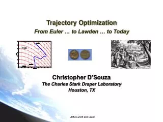
Trajectory Optimization From Euler … to Lawden … to Today. Christopher D’Souza The Charles Stark Draper Laboratory Houston, TX. Why Optimize?. Engineers are always interested in finding the ‘best’ solution to the problem at hand Fastest Fuel Efficient

E N D
Trajectory OptimizationFrom Euler … to Lawden … to Today Christopher D’Souza The Charles Stark Draper Laboratory Houston, TX
Why Optimize? • Engineers are always interested in finding the ‘best’ solution to the problem at hand • Fastest • Fuel Efficient • Optimization theory allows engineers to accomplish this • Often the solution may not be easily obtained • In the past, it has been surrounded by a certain mystique • This seminar is aimed at demystifying trajectory optimization • Practical trajectory optimization is now within reach • State of the art computers • State of the art algorithms • In order to fully appreciate trajectory optimization, however, one must understand something about it’s history • We need to understand where we’ve been in order to appreciate where we are
The Greeks started it! • Queen Dido of Carthage (7 century BC) • Daughter of the king of Tyre • Fled Tyre to Tunisia • Agreed to buy as much land as she could “enclose with one bull’s hide” • Set out to choose the largest amount of land possible, with one border along the sea • A semi-circle with side touching the ocean • Founded Carthage • Fell in love with Aeneas but committed suicide when he left • Story immortalized in Homer’s Aeneid
The Italians Countered • Joseph Louis Lagrange (1736-1813) • His work Mécanique Analytique (Analytical Mechanics) (1788) was a mathematical masterpiece • Invented the method of ‘variations’ which impressed Euler and became ‘calculus of variations’ • Invented the method of multipliers (Lagrange multipliers) • Sensitivities of the performance index to changes in states/constraints • Became the ‘father’ of ‘Lagrangian’ Dynamics • Euler-Lagrange Equations • Obtained the equilibrium points of the Earth-Moon and Earth-Sun system
The Multi-Talented Mr. Euler • Euler (1707-1783) • Friend of Lagrange • Published a treatise which became the de facto standard of the ‘calculus of variations’ • The Method of Finding Curves that Show Some Property of Maximum or Minimum • He solved the brachistachrone (brachistos = shortest, chronos = time) problem very easily • Minimum time path for a bead on a string • Cycloid
The Plot Thickens: Hamilton and Jacobi • William Hamilton (1805-1865) • Published work on least action in mechanical systems that involved two partial differential equations • Inventor of the quaternion • Karl Gustav Jacob Jacobi (1804-1851) • Discovered ‘conjugate points’ in the fields of extremals • Gave an insightful treatment to the second variation • Jacobi criticized Hamilton’s work • Only one PDE was required • Hamilton-Jacobi equation • Became the basis of Bellman’s work 100 years later
The ‘Chicago School’ • At the beginning of the twentieth century Gilbert Bliss and Oskar Bolza gathered a number of mathematicians at the University of Chicago • Made major advances in calculus of variations following on the work of Karl Wilhelm Theodor Weierstrass • Applied this to the field of ballistics during WW I • Artillery firing tables • Second Variation Conditions (conjugate point conditions) • Built on the work of Legendre, Jacobi, and Clebsch • Graduated many of the premiere applied mathematicians of the early/mid 20th century • M. R. Hestenes • E. J. McShane
Derek and the Primer • During the 1950s, Derek Lawden applied the calculus of variations to exo-atmospheric rocket trajectories • Published Optimal Space Trajectories for Navigation • Concerned with thrusting and coasting arcs • ‘Invented’ the primer vector • Direction is along the thrust direction • Directly related to the velocity Lagrange multiplier • Provided a methodology for determining optimal space trajectories
The Russians are Coming – Pontryagin • In the mid 1950s a group of Russian Air Force officers went to the Steklov Mathematical Institute outside of Moscow to find out whether the mathematicians could determine a particular set of optimal aircraft maneuvers • Pontryagin, the director of the Institute, accepted the challenge and went on to invent a ‘new calculus of variations’ • The Maximum Principle • Used the concept of control parameters, upravlenie, or u • Solved the original problem and in the process revolutionized optimal control and trajectory optimization
The American Response – Bryson • Arthur Bryson, then at Harvard, an aerodynamicist, came across the paper by Pontryagin and immediately recognized its value • He applied it to a problem of finding an minimum time to climb trajectory and presented it to the military • It was sent to Pax River and was demonstrated by Lt. John Young (using an altitude vs Mach number table at 1000 ft intervals) • 338 seconds vs the predicted 332 seconds • Path • Accelerate to M = 0.84 at just about ground level where drag rise begins • Climb at constant Mach number to 30,000 ft • Shallow dive to 24,000 ft followed by a slow climb to 30000 ft, increasing energy until the energy equals the final energy • Climb very rapidly to desired altitude (20 km) • Applied this new ‘optimal control theory’ to various aerospace engineering problems, particularly those of interest to the US military
The Inescapable Kalman • Rudolf Kalman first came on the scene in the late 50s leading the way to the state space paradigm of control theory along with the concepts of controllability and observability • He then introduced an integral performance index that had quadratic penalties on the state error and control magnitude • Demonstrated that the optimal controls were linear feedbacks of the state variables • Led to time varying linear systems and MIMO systems • He later collaborated with Bucy to give us the Kalman-Bucy filter As some may know, these concepts were integral to the success of the guidance and navigation systems on the Apollo program
Other Trajectory Optimization Legends • Richard Bellman • Introduced a new view and an extension of Hamilton-Jacobi theory called Dynamic Programming and the Hamilton-Jacobi-Bellman equation • Led to a family of extremal paths • Provides optimal nonlinear feedback • Curse of dimensionality • John Breakwell • Among the first to apply the calculus of variations to optimal spacecraft and missile trajectories • Prof. Angelo Miele • Among the first to develop numerical procedures for solving trajectory optimization problems (SGRA) • Dr. Henry (Hank) Kelly • Developed conditions for singular optimal control problems (called the Kelley Conditions in Russia)
So What? • The brief reconnaissance into the history of trajectory optimization is intended to demonstrate the rich heritage which we possess • It was also intended to prepare us for a discussion of where we are and where we are going • We began this seminar asking the question: Why optimize? • Because we are engineers and we want to find the ‘best’ solution • So, how do we go about optimizing?
What to Optimize? • Engineers intuitively know what they are interested in optimizing • Straightforward problems • Fuel • Time • Power • Effort • More complex • Maximum margin • Minimum risk • The mathematical quantity we optimize is called a cost function or performance index
The Trajectory Optimization Nomenclature • Dynamical constraints • Examples: equations of motion (Newton’s Laws) • Controls (u) • Exogenous (independent) variables which operate on the system • Examples: Thrust, flight control surfaces • States (x) • Dependent variables which define the ‘state’ of the system • Examples: position, velocity, mass • Terminal constraints • Conditions that the initial and final states must satisfy • Example: circular orbit with a particular energy and inclination • Path constraints • Conditions which must be satisfied at all points of the trajectory • Example: Thrust bounds • Point constraints • Conditions at particular points along the trajectory • Examples: way points, maximum heating • Trajectory optimization seeks to obtain both the states and the controls which optimize the chosen performance index while satisfying the constraints
The Optimal Control Problem The general trajectory optimization problem can be posed as: find the states and controls which subject to the dynamics which takes the system from to the terminal constraints
The Optimality Conditions and Pontryagin’s Minimum Principle These are also called the Euler-Lagrange equations
The Optimality Conditions and Pontryagin’s Minimum Principle The boundary conditions are There is one additional condition (sometimes called the Weierstrass Condition) which must satisfy for any (the set of controls that meet the constraints) All of these conditions are collectively called the Pontryagin Minimum Principle (PMP)
Comments on the Pontryagin Minimum Conditions • The Pontryagin conditions are very powerful tools to help find optimal trajectories • Infinite Dimensional Conditions • It is a two-point boundary value problem • States are specified at the initial time • Costates (Lagrange multipliers) are specified at the final time • Some states (or combinations of states) are specified at the final time • Equivalent to solving a PDE • Most problems cannot be solved in closed form • Closed form solutions lend themselves to analysis • Need to use numerical methods to obtain solutions for real-world problems • No guarantee of a solution • Convergence issues • Stability issues • In the process we convert an infinite dimensional problem into a finite dimensional problem • Implicit in numerical integration
How to Optimize? • Two general types of methods exist for solving optimal control problems • Direct Methods • Discretize the states and controls at points in time • Nodes • Convert the problem into a parameter optimization problem • States and controls at the nodes become the optimizing parameters • Use an NLP (Non-Linear Program) to solve the parameter optimization problem • Advantages: Fast Solution • Disadvantages: Difficult to determine/prove optimality • Indirect Methods • Operate on the Pontryagin Necessary Conditions • This is a two-point boundary value problem • Use Shooting methods • Advantages: Easy to determine optimality • Disadvantages: (Very) difficult to converge
x t Direct Methods • Collocation • A method in which you choose states and controls at points in time along the trajectory • These points are called nodes • States and control values at the nodes become the optimizing variables • Convert the infinite dimensional problem into a finite dimensional, parameter optimization problem • Enforce the constraints at the nodes • Dynamic • Path • Solved using a NonLinear Program (NLP) • Types of Spacing • Uniform spacing • Nonuniform spacing
Numerical Optimization Solvers • The general form of the nonlinear programming problem (NLP) is • My favorite is SNOPT developed by Philip Gill • Sparse sequential quadratic programming (SQP) • Can be used for problems with thousands of constraints and variables • State of the art
Trajectory Optimization Packages • POST (Program to Optimize Simulated Trajectories) • Direct/Multiple shooting FORTRAN program originally developed in 1970 for Space Shuttle Trajectory Optimization by NASA Langley • Generalized point mass, discrete parameter targeting and optimization program. • Provides the capability to target and optimize point mass trajectories for a powered or unpowered vehicle near an arbitrary rotating, oblate planet • SORT (Simulation and Optimization Rocket Trajectories) • FORTRAN program originally developed for ascent vehicle trajectories • Used to generate Space Shuttle guidance targets and maintained by Lockheed-Martin • Can be used with a optimization package to optimize the trajectory • Variable Metric Methods • NPSOL • OTIS (Optimal Trajectories through Implicit Simulation) • FORTRAN program for simulating and optimizing point mass trajectories of a wide variety of aerospace vehicles from NASA Glenn supported by Boeing (Steve Paris) in Seattle • Originally developed by Hargraves and Paris • Designed to simulate and optimize trajectories of launch vehicles, aircraft, missiles, satellites, and interplanetary vehicles • Can be used to analyze a limited set of multi-vehicle problems, such as a multi-stage launch system with a fly back booster • Hermite-Simpson collocation method which uses NZOPT as NLP
State of the Art Optimizers for Optimal Control • SOCS (Sparse Optimization for Control Systems) • General-purpose FORTRAN software for solving optimal control problems from Boeing (Seattle) • Trajectory optimization • Chemical process control • Machine tool path definition • Uses Trapezoid, Hermite-Simpson or Runge-Kutta integration • NLP is SPRNLP written by Betts and Huffman • Uniform node spacing, but can have multiple intervals • Provides mesh refinement for complex problems • DIDO (Direct and InDirect Optimization) • Also named after Queen Dido of Carthage • General-purpose user-friendly MATLAB software for solving optimal control problems from NPS • Non-uniform node spacing with multiple intervals • Legendre-Gauss-Lobatto points • Uses a sparse numerical optimization solver (SNOPT) • Can determine if the necessary conditions are satisfied • Has been used to solve a wide variety of missile and spacecraft problems • Very fast even for complex problems • Current research is being directed toward real-time uses
The Wave of the Future – Pseudospectral Methods • Pseudospectral methods choose the collocation points in such a way as to minimize integration error • Number of nodes dependent on accuracy desired • The nodes are non-uniformly spaced in time • Quadratic spacing at the ends • Number determines the spacing • They use (global basis) functions which (optimally) approximate the states and controls and enforce the (dynamic and path) constraints at the nodes over the interval [-1, 1] • Chebyshev-Gauss • Legendre-Gauss • Chebyshev-Gauss-Lobatto • Legendre-Gauss-Lobatto • Pseudospectral methods yield ‘spectral accuracy’ • Optimal interpolation • Particularly well suited for trajectory optimization problems where much of the activity occurs at the ends of the intervals } Includes the end points
Pseudospectral Point Distribution (N = 10) } } Quadratic clustering at ends
Suppose we wish to find the optimal trajectory for a three stage vehicle to get the maximum payload to orbit Performance index Differential constraints (equations of motion) Terminal constraints Throttle capability (minimum, maximum specified) Coast of at least 5 seconds between second and third stage Maximum of 115 seconds Launch Vehicle Example: Three Stage to Orbit
Problem Specific Issues • Coordinate Systems • Dynamics • Inertial • Spherical • Equinoctial • Controls • Angles • Thrust components • Direction cosines • Scaling • For good convergence properties, we need all the variables to be of ‘order 1’ • So we scale the states, the controls and the time to achieve this • The ‘art’ of trajectory optimization • Tuning knobs
Three Stage to Orbit Thrust Profile Maximum Thrust Minimum Thrust Coast
Three Stage to Orbit Thrust Direction Profile Second Stage Separation First Stage Separation
Three Stage to Orbit Mass Profile First Stage Separation Second Stage Separation Coast
Orbit Transfer • Optimal transfers between two orbits have been the subject of directed research for the past 40 years • Much analytical and computational effort has been devoted to this task • Primer vector theory has been applied • Numerical solutions are sometimes difficult to obtain • The Legendre PseudoSpectral (LPS) method has been used to extensively analyze this problem • Impulsive burn approximations • Finite burn effects • Types of coordinate systems • Cartesian • Equinoctial • Nonsingular orbital elements
Impulsive Orbit Transfer Elliptical-Elliptical Transfer with Inclination Change Analytic Solution: v1= 2106.13 m/s v2 = 239.69 m/s LPS Solution: v1= 2106.17 m/s v2 = 239.65 m/s Elliptical-Elliptical Hohmann Transfer Analytic Solution: v1= 2076.72 m/s v2 = 87.46 m/s LPS Solution: v1= 2076.71 m/s v2 = 87.49 m/s
Finite Burn Orbit Transfer: LEO (ISS) to LEO (Sun Synchronous) • Finite Burn Accumulated DV • DV = 8027.5 m/s • Impulsive Burn Accumulated DV • DV = 6548.6 m/s
Further Applications of LPS • ISS Momentum Desaturation • Constellation Design • Libration point formation designs • Entry Trajectory Design • Planetary Mission Design
What is Next? -- MAHC • Multi-Agent Hybrid Control (MAHC) • 21st Century extension of 20th Century optimal control • A general optimization framework for multiple vehicles • Multiple constraints on each vehicle • Allow for discrete decision variables • Example • Two stage vehicle • Return vehicle must land at a particular point • Latitude: -28.25N § 1 km • Longitude: -70.1 E § 1 km • Ascent vehicle continues to a desired orbit while maximizing mass to orbit • The discrete state space is as follows
Multi-Agent Hybrid Trajectory Optimization Example: Position Profile
What is Next? -- Real-time Trajectory Optimization • ‘Real-time’ trajectory optimization • Computational capability is increasing with Moore’s law • Time is approaching when these (direct) methods can be implemented on board vehicles and optimized in ‘real-time’ • 1 Hz • Guidance cycles (outer loop) slower than control cycles (inner loop) • Application to orbit (transfer) problem • Issues • Convergence • Stability of solutions
What is Next? - NOG • Neighboring Optimal Guidance (NOG) • A real-time guidance scheme which determines a new optimal path which is ‘close’ to the nominal (a priori) optimal path • Neighboring optimal • Operates on deviations from the optimal trajectory • Very robust • Based upon the second variation sufficient conditions
Conclusion • Trajectory optimization has advanced greatly over the past 40 years • We are at the threshold of a new era for solving exciting complex optimization problems • New methods exist for solving (general) optimal control problems • Trajectory optimization problems are a subset of this class • These methods give (reasonably) fast solutions even given poor guesses • Fast computers • Good algorithms • Don’t need to know the details of the methods or devote your career to optimization • Just your problem • Solution of complex trajectory optimization problems is within reach of the practicing engineer
Selected References • Lietmann, G., Optimization Techniques, Academic Press, 1962. • Lawden, D.F., Optimal Trajectories for Space Navigation, Butterworths, 1963. • Bryson, A.E. and Ho, Y-C., Applied Optimal Control, Hemisphere Publishing Company, 1975. • Gill, P.E., Murray, W., and Wright, M.H., Practical Optimization, Academic Press, 1981. • Fletcher, R., Practical Methods of Optimization, Wiley Press, 1987. • Betts, J.T., Practical Methods for Optimal Control Using Nonlinear Programming, SIAM: Advances in Control and Design Series, 2001.