Download
1 / 10
100 likes | 254 Views
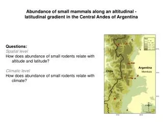
Abundance of small mammals along an altitudinal - latitudinal gradient in the Central Andes of Argentina. Questions : Spatial level How does abundance of small rodents relate with altitude and latitude? Climatic level How does abundance of small rodents relate with climate?. Spatial level.

E N D
Abundance of small mammals along an altitudinal - latitudinal gradient in the Central Andes of Argentina Questions: Spatial level How does abundance of small rodents relate with altitude and latitude? Climatic level How does abundance of small rodents relate with climate?
Spatial level We explore the data in a graphical way xyplot(ABUND~ALT|lat,groups=lat,type="b",lwd=3) 34°LAT 35°LAT A B U N D A N C E 32°LAT 33°LAT ALTITUDE
Spatial level Bar plot of abundance variation per altitude for each latitude. a=with(an,tapply(ABUND,list(ALT,lat),mean)) barplot(a,beside=TRUE) Abundance peaks at 2300m. We observed a quadratic relationship. A B U N D 2300 1800 3300 2800 1300 lat
Spatial level We rescaled the latitude and altitude axes: alt=((ALT-1300)/1000)# to standardize the variable lt=(lat-32) We transformed abundance to log, to get a better fit to a normal distribution. ab=log(ABUND) We performed a linear model:Spatial Model =lm(ab~lt+alt+I(lt^2)+I(alt^2)) Coefficients: Estimate Std. Error t value Pr(>|t|) (Intercept) 2.5076 0.4542 5.521 5.87e-05 *** lt 1.1659 0.5288 2.2050.04350 * alt 3.3662 0.8422 3.9970.00117 ** I(lt^2) -0.3981 0.1689 -2.3570.03246 * I(alt^2) -1.4410 0.4038 -3.5680.00280 ** Signif. codes: 0 ‘***’ 0.001 ‘**’ 0.01 ‘*’ 0.05 ‘.’ 0.1 ‘ ’ 1 Residual standard error: 0.7555 on 15 degrees of freedom Multiple R-squared: 0.5993, Adjusted R-squared: 0.4924 F-statistic: 5.608 on 4 and 15 DF, p-value: 0.005772
Spatial level Lollipop3d graph showing the relationship between log-abundance and the spatial predictor variables, altitude and latitude. Log(abund)=latitude+altitude+latitude2+altitude2 Abundance shows a hump shape pattern along altitude (peak= 2300m) and latitude (peak= 33° S).
Climatic level Climatic variables: we reduced the variability of all precipitation variables into one PCA (Prec) and all temperature variables into one PCA (Temp). Temperature seasonality accounts for 94% of the variation in PCA (Temp). PCA Annual mean precipitation (53%), Precipitation of the wettest season (20%) and Precipitation of the coldest season (20%) accounts for 93% of the variation in PCA (Prec). Log abundance has a quadratic relationship with the climatic variables.
Climatic level We performed a Linear model: Climatic model=lm(log(ABUND)~PCA_Temp+PCA_Prec+I(PCA_Temp^2)+I(PCA_Prec^2)) Coefficients: Estimate Std. Error t value Pr(>|t|) (Intercept) 4.805e+00 2.844e-01 16.895 3.58e-11 *** PCA_Temp -1.027e-04 7.380e-04 -0.139 0.8912 PCA_Prec 1.117e-03 1.278e-03 0.874 0.3958 I(PCA_Temp2) -3.528e-06 1.650e-06 -2.138 0.0494 * I(PCA_Prec2) -1.153e-05 5.416e-06 -2.129 0.0502 . Signif. codes: 0 ‘***’ 0.001 ‘**’ 0.01 ‘*’ 0.05 ‘.’ 0.1 ‘ ’ 1 Residual standard error: 0.8337 on 15 degrees of freedom Multiple R-squared: 0.512, Adjusted R-squared: 0.3819 F-statistic: 3.934 on 4 and 15 DF, p-value: 0.02229
Climatic level Lollipop3d graph showing the relationship between log-abundance and the climatic predictor variables, PCA (Temp), PCA (Prec). Abundance is maximum at intermediate values of temperature and precipitation. Annual mean precipitation Precipitation of the wettest season Precipitation of the coldest season Temperature Seasonality
Final remarks We compared the spatial and climatic model using the Akaike’s Information Criterion AIC df dAIC Weight Spatial model 51.8 6 0.0 0.878 Climatic model 55.7 6 3.9 0.122 The spatial fits better than the climatic model. Apparently altitude variability is composed by more than climatic variables. Conclusion: How does abundance of small rodents relate with altitude and latitude? In a quadratic relationship, with a peak at intermediate altitudes and latitudes. How does abundance of small rodents relate with climate? In a quadratic relationship peaking at intermediate Temperature Seasonality and Precipitation.