Download
1 / 76
2.06k likes | 3.57k Views
Digital Image Processing Chapter 3: Image Enhancement in the Spatial Domain 15 June 2007. Spatial Domain. What is spatial domain. The space where all pixels form an image. In spatial domain we can represent an image by f(x,y) where x and y are coordinates along x and y axis with

E N D
Digital Image Processing Chapter 3: Image Enhancement in the Spatial Domain 15 June 2007
Spatial Domain What is spatial domain The space where all pixels form animage In spatial domain we can represent animageby f(x,y) wherex andy are coordinates along x and y axis with respect to an origin There is duality betweenSpatial andFrequency Domains Usingthe Fourier transform, the word “distance” is lost but the word “frequency” becomes alive. Images in the spatial domain are pictures in thexyplane where the word “distance” is meaningful.
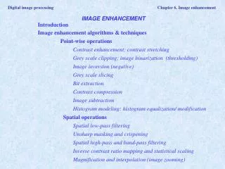
Image Enhancement Image Enhancement means improvement of images to be suitable for specific applications. Example: Note: each image enhancement technique that is suitable for one application may not be suitable for other applications. (Images from Rafael C. Gonzalez and Richard E. Wood, Digital Image Processing, 2nd Edition.
Image Enhancement Example Original image Enhanced image using Gamma correction (Images from Rafael C. Gonzalez and Richard E. Wood, Digital Image Processing, 2nd Edition.
Image Enhancement in the Spatial Domain = Image enhancement using processes performed in the Spatial domainresulting in images in theSpatial domain. We can written as wheref(x,y) is an original image, g(x,y) is an output and T[ ] isa function defined in the area around(x,y) Note: T[ ] may haveone input asa pixel value at(x,y) only or multiple inputsaspixels inneighbors of(x,y) depending in each function. Ex. Contrast enhancement uses apixel value at (x,y) only for an input while smoothing filte use several pixels around (x,y) as inputs.
Types of Image Enhancement in the Spatial Domain - Single pixel methods - Gray level transformations Example - Historgram equalization - Contrast stretching - Arithmetic/logic operations Examples - Image subtraction - Image averaging - Multiple pixel methods Examples Spatial filtering - Smoothing filters - Sharpening filters
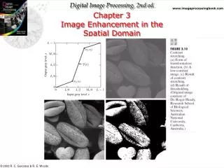
Gray Level Transformation Transformsintensity of an original image intointensity of an output image using a function: wherer =input intensity ands =output intensity Example: Contrast enhancement (Images from Rafael C. Gonzalez and Richard E. Wood, Digital Image Processing, 2nd Edition.
Image Negative L-1 Original digital mammogram White Output intensity Negative digital mammogram Black 0 L-1 Black White Input intensity L = the number of gray levels (Images from Rafael C. Gonzalez and Richard E. Wood, Digital Image Processing, 2nd Edition.
Log Transformations Application Fourier spectrum Log Tr. of Fourier spectrum (Images from Rafael C. Gonzalez and Richard E. Wood, Digital Image Processing, 2nd Edition.
Power-Law Transformations (Images from Rafael C. Gonzalez and Richard E. Wood, Digital Image Processing, 2nd Edition.
Power-Law Transformations : Gamma Correction Application Image displayed at Monitor Desired image Image displayed at Monitor After Gamma correction (Images from Rafael C. Gonzalez and Richard E. Wood, Digital Image Processing, 2nd Edition.
Power-Law Transformations : Gamma Correction Application MRIImage after Gamma Correction (Images from Rafael C. Gonzalez and Richard E. Wood, Digital Image Processing, 2nd Edition.
Power-Law Transformations : Gamma Correction Application Ariel images afterGamma Correction (Images from Rafael C. Gonzalez and Richard E. Wood, Digital Image Processing, 2nd Edition.
Contrast Stretching Contrast means the difference between the brightest and darkest intensities Before contrast enhancement After (Images from Rafael C. Gonzalez and Richard E. Wood, Digital Image Processing, 2nd Edition.
How to know where the contrast is enhanced ? • Notice the slope ofT(r) • ifSlope > 1 Contrast increases • ifSlope < 1 Contrast decrease • ifSlope = 1 no change Ds Dr Smaller Dr yieldswider Ds = increasing Contrast (Images from Rafael C. Gonzalez and Richard E. Wood, Digital Image Processing, 2nd Edition.
Gray Level Slicing (Images from Rafael C. Gonzalez and Richard E. Wood, Digital Image Processing, 2nd Edition.
Bit-plane Slicing Bit 7 Bit 6 Bit 5 Bit 3 Bit 2 Bit 1 (Images from Rafael C. Gonzalez and Richard E. Wood, Digital Image Processing, 2nd Edition.
Histogram Histogram = Graph of population frequencies Grades of the course 178 xxx
Histogram of an Image = graph ofno. of pixels vs intensities Dark image has histogram on the left จำนวน pixel Bright image has histogram on the right จำนวน pixel (Images from Rafael C. Gonzalez and Richard E. Wood, Digital Image Processing, 2nd Edition.
Histogram of an Image (cont.) low contrastimage has narrowhistogram high contrastimage has widehistogram (Images from Rafael C. Gonzalez and Richard E. Wood, Digital Image Processing, 2nd Edition.
Histogram Processing =intensity transformation based onhistogram information to yield desired histogram - Histogram equalization To makehistogram distributed uniformly - Histogram matching To makehistogram as the desire
Monotonically Increasing Function =Function that is only increasing or constant Properties of Histogram processing function 1.Monotonically increasing function 2.
Probability Density Function Histogram is analogous toProbability Density Function (PDF)which represent density of population Lets andr beRandom variables withPDFps(s) andpr(r ) respectively and relation betweens andris We get
Histogram Equalization Let We get !
Histogram Equalization Formula in the previous slide is fora continuous PDF ForHistogram ofDigital Image, we use nj = the number of pixels with intensity = j N = the number of total pixels
Histogram Equalization (Images from Rafael C. Gonzalez and Richard E. Wood, Digital Image Processing, 2nd Edition.
Histogram Equalization (cont.) (Images from Rafael C. Gonzalez and Richard E. Wood, Digital Image Processing, 2nd Edition.
Histogram Equalization (cont.) (Images from Rafael C. Gonzalez and Richard E. Wood, Digital Image Processing, 2nd Edition.
Histogram Equalization (cont.) (Images from Rafael C. Gonzalez and Richard E. Wood, Digital Image Processing, 2nd Edition.
Histogram Equalization (cont.) Original image Afterhistogram equalization, the image become a low contrast image (Images from Rafael C. Gonzalez and Richard E. Wood, Digital Image Processing, 2nd Edition.
Histogram Matching: Algorithm To transformimage histogram to be a desired histogram Concept: fromHistogram equalization, we have We get ps(s) = 1 We want an output image to havePDFpz(z) Apply histogram equalization topz(z), we get We getpv(v) = 1 Sinceps(s) = pv(v) = 1 therefores andv are equivalent Therefore, we can transformr toz by T( ) G-1( ) r s z
Histogram Matching : Algorithm (cont.) s = T(r) v = G(z) 2 1 3 z = G-1(v) 4 (Images from Rafael C. Gonzalez and Richard E. Wood, Digital Image Processing, 2nd Edition.
Histogram Matching Example Input image histogram Desired Histogram Example Original data User define
Histogram Matching Example (cont.) 1. ApplyHistogram Equalization to both tables sk = T(rk) vk = G(zk)
Histogram Matching Example (cont.) 2. Get amap Actual Output Histogram We get r s v z s v sk = T(rk) zk = G-1(vk)
Histogram Matching Example (cont.) Desired histogram Transfer function Actual histogram (Images from Rafael C. Gonzalez and Richard E. Wood, Digital Image Processing, 2nd Edition.
Histogram Matching Example (cont.) After histogram equalization After histogram matching Original image
Local Enhancement : Local Histogram Equalization Concept: Perform histogram equalization in a small neighborhood After Local Hist Eq. In 7x7 neighborhood Orignal image After Hist Eq. (Images from Rafael C. Gonzalez and Richard E. Wood, Digital Image Processing, 2nd Edition.
Local Enhancement : Histogram Statistic for Image Enhancement We can use statistic parameters such asMean, Variance ofLocal area for image enhancement Image of tungsten filament taken using An electron microscope In the lower right corner, there is a filament in the background which is very dark and we want this to be brighter. We cannot increase the brightness of the whole image since the white filament will be too bright. (Images from Rafael C. Gonzalez and Richard E. Wood, Digital Image Processing, 2nd Edition.
Local Enhancement Example:Local enhancement for this task Local Variance image Multiplication factor Original image (Images from Rafael C. Gonzalez and Richard E. Wood, Digital Image Processing, 2nd Edition.
Local Enhancement Output image (Images from Rafael C. Gonzalez and Richard E. Wood, Digital Image Processing, 2nd Edition.
Logic Operations Application: Crop areas of interest AND OR Original image Result Region of Interest Image mask (Images from Rafael C. Gonzalez and Richard E. Wood, Digital Image Processing, 2nd Edition.
Arithmetic Operation: Subtraction Application: Error measurement Error image (Images from Rafael C. Gonzalez and Richard E. Wood, Digital Image Processing, 2nd Edition.
Arithmetic Operation: Subtraction (cont.) Application: Mask mode radiography in angiography work (Images from Rafael C. Gonzalez and Richard E. Wood, Digital Image Processing, 2nd Edition.
Arithmetic Operation: Image Averaging Application : Noise reduction Degraded image (noise) Image averaging Averaging results inreduction of Noise variance (Images from Rafael C. Gonzalez and Richard E. Wood, Digital Image Processing, 2nd Edition.
Arithmetic Operation: Image Averaging (cont.) (Images from Rafael C. Gonzalez and Richard E. Wood, Digital Image Processing, 2nd Edition.
Basics of Spatial Filtering Sometime we need to manipulate values obtained from neighboring pixels Example: How can we compute an average value of pixels in a 3x3 region center at a pixel z? Pixel z 2 4 1 2 6 2 9 2 3 4 4 4 7 2 9 7 6 7 5 2 3 6 1 5 7 4 2 5 1 2 2 5 2 3 2 8 Image
Basics of Spatial Filtering (cont.) Step 1. Selected only needed pixels Pixel z … 2 4 1 2 6 2 9 2 3 4 4 4 3 4 4 … … 7 2 9 7 6 7 9 7 6 5 2 3 6 1 5 3 6 1 7 4 2 5 1 2 … 2 5 2 3 2 8