Download
1 / 44
440 likes | 625 Views
Physical Based Modeling and Animation of Fire and Water Surface. Presented at Prof. Joe KeaRney’s animation lecture. Jun Ni, Ph.D. M.E. Associate Research Scientist, Research Services Adjunct Assistant Professor Department of Computer Science Department of Mechanical Engineering.

E N D
Physical Based Modeling and Animation of Fire and Water Surface Presented at Prof. Joe KeaRney’s animation lecture Jun Ni, Ph.D. M.E. Associate Research Scientist, Research Services Adjunct Assistant Professor Department of Computer Science Department of Mechanical Engineering
Dr. Ronald Fediw Department of Computer Science, Stanford University Conference proceeding at ACM SIGGRAPH 2002
Animation of FireOutline • Introduction • Physical Based Model • Level-set Implementation • Rendering of Fire • Animation Results
Introduction • Modeling of natural phenomena such as fire and water remains a challenging problem in computer graphics • Complications of the modeling • fluid motion with un-stability, transient, non-linear, multi-phases, and multi-component, combustion (chemical reactions), different physical scales, fluid compression, explosions and wave • For example, fluid reaction system • Combustion processes can be classified into two distinct types of phenomena • Detonations • Deflagrations
Introduction to physical phenomena • Deflagrations : low speed events with chemical reactions converting fuel into hot gaseous products, such as fire and flame. They can be modeled as an incompressible and inviscid (less viscous) flow • Detonations: high speed events with chemical reactions converting fuel into hot gaseous productions with very short period of time, such as explosions (shock-wave and compressible effects are important)
Introduction to Modeling • How to model? • Introduce a dynamic implicit surface to track the reaction zone where the gaseous fuel is converted into the hot gaseous products • The gaseous fuel and hot gaseous zones are modeled separately by using independent sets of incompressible flow equations. • Coupling the separate equations by considering the mass and momentum balances along the reaction interface (the surface)
Introduction to Modeling • How to model? • Rendering the fire as a participating medium with black body radiation using stochastic ray marching algorithm • Chromatic adaptation of observer to get the reaction colors of the fire
Physical Based Model • Three distinct visual phenomena: • Blue or bluish-green core: emission lines from intermediate chemical species, such as carbon radical generated during reaction. It is located adjacent to the implicit surface imposed. this color can be used to track the movement of the surface • Yellowish-orange color: blackbody radiation emitted by the hot gaseous products (carbon soot) • Fire soot or smoke core: temperature cools to the point where the blackbody radiation is no longer visible
Temperature blue core T max gas fuel ignition solid fuel gas products gas to solid phase change time
Soot emit blackbody radiation that illuminates smoke Hot gaseous products Blue core
Physical Based Model • Blue or bluish-green core: • surface area of the blue core is determined by vfAf =SAs Vf is the speed of fuel injected, Af is the cross section area of cylindrical injection Reacted gaseous fuel S As Implicit surface Af Un-reacted gaseous fuel vf
S is small and core is large S is large and core is small Blue reaction zone cores with increased speed S (left); with decreased speed S (right)
Physical Based Model • Premixed flame and diffusion flame • fuel and oxidizer are premixed and gas is ready for combustion • non-premixed (diffusion) premixed flame diffusion flame oxidizer fuel fuel Location of blue reaction zone
Physical Based Model • Hot Gaseous Products • Expansion parameter rf/rh rf=1.0 rh=0.2 0.1 0.02
Physical Based Model • Mass and momentum conservation require rh(Vh-D)=rf(Vf-D) rh (Vh-D)2 +ph = rf(Vf-D)2+pf Vf and Vh are the normal velocities of fuel and hot gaseous D =Vf-S speed of implicit surface direction
Physical Based Model • Solid fuel • Use boundary as reaction front Vf=Vs+(rs /rf-1)S rs and Vs are the density and the normal velocity of solid fuel Solid fuel
Implementation • Discretization of physical domain into N3 voxels (grids) with uniform spacing • Computational variables implicit surface, temperature, density, and pressure, fi,j,k, Ti,j,k, ri,j,k, and pi,j,k • Track reaction zone using level-set methods, f=+,-, and 0, representing space with fuel, without fuel, and reaction zone • Implicit surface moves with velocity w=uf+sn, so the surface can be governed by ft= - w f
Implementation • Incompressible flow for gaseous fuel and hot gaseous product zone ut= - (u ) u - p/r +a(T-Tair)z u=0 p/r ) = u*/ t (
Implementation • Temperature and density • T=Tignition for blue zone • Linear interpolation between Tignition and Tmax for hot gaseous product zone • Energy conservation T-Tair 4 T = - (u ) T – Ct ( ) Tmax-Tair
Rendering of Fire • Fire: participating medium • Light energy • Bright enough to our eyes adapt its color • Chromatic adaptation • Approaches • Simulating the scattering of the light within a fire medium • Properly integrating the spectral distribution of the power in the fire and account for chromatic adaptation
Rendering of Fire • Light Scattering in a fire medium • Fire is a blackbody radiator and a participating medium • Properties of participating are described by • Scattering and its coefficient • Absorption and its coefficient • Extinction coefficient • Emission • These coefficients specify the amount of scattering, absorption and extinction per unit-distance for a beam of light moving through the medium
Rendering of Fire • Phase function p(g, w) is introduced to address the distribution of scatter light, where g(-1,0) (for backward scattering anisotropic medium) g(0) (isotropic medium), and g(0,1) (for forward scattering anisotropic medium) • Light transport in participating medium is described by an integro-differential equation Emitted radiance w Ll(x,w)=f(coefficients, Ll, Lel, w) Incoming direction angle of scattering light Spectral radiance
Rendering of Fire • Reproducing the color of fire • Full spectral distribution --- using Planck’s formula for spectral radiance in ray machining • The spectrum can be converted to RGB before being displaying on a monitor • Need to computer the chromatic adaptation for fire --- hereby using a transformation Fairchild 1998)
Rendering of Fire • Reproducing the color of fire • Assumption: eye is adapted to the color of the spectrum for maximum temperature presented in the fire • Map the spectrum of this white point to LMS cone responsivities (Lw, Mw, Sw) (Fairchild ‘s book “color appearance model”, 1998) (Xa, Ya, Za) (Xr, Yr, Zr) Adapted XYZ tristimulus values raw XYZ tristimulus values
Animation Result • Domain: 8 meters long with 160 grids (increment h=0.05m) • Vf=30m/s Af=0.4m • S=0.1m/s • rf=1 • rh=0.01 • Ct=3000K/s • a=0.15 m/(Ks2)
A flammable ball passes through a gas flame and catches on fire It is time to see several animations!
Animation of WaterOutline • Introduction • Physical Based Simulation Model • Particle -Level-set Method • Rendering of Water • Animation Results
Introduction • Photorealistic simulation of water surface • Treatment of the surface separating the water from air • Two-phase problem • Providing visual impression of water with surface • Key point is to model the surface • Approach: particle level-set method
Introduction • Particle level-set method • Hybrid surface tracking method using mass-less marker particles combined with a dynamic implicit surface • An implicit surface imposed to representing water surface during computation.
Introduction • Particle level-set method • Velocity extrapolation procedure across the water surface into the region occupied by the air. • Control the behavior of water surface • Add dampening and/or churning effects
Introduction • Rendering of water • Relatively easy, since it optical properties are well understood and can be well described. • Surface tension caused illumination • There are several algorithms • Path tracing • Bidirectional path tracing • Metropilis light transport • Photon mapping
Simulation Methods • Liquid volume model (previous model) • Implicit function, f (<0 water, >0 air, =0 surface) (Foster and Fedkiw, 2001) ft + u f = 0 Particle motion transport equation
Using previous model Using modified model
Simulation Methods • Particle Level-set model (modified or particle enhanced level-set model) • Impose two sets (positive and negative particles) on both sides of fluid regions separated by the implicit surface
Simulation Methods • Radius of particle changes dynamics throughout the simulation and is based on level-set function f. rmax if spf(xp)>rmax rp ={ spf(xp) rmin<spf(xp)<rmax rmin if spf(xp)<rmin Sign function (1 for positive particle and -1 for negative particle)
Simulation Methods • Extrapolation method for air motion • ut = -N u u is velocity in x component Unit velocity perpendicular to the implicit surface N
Simulation Methods • equation for fluid motion (N-S) • ut = -u 1 u+ n ( u) - p +g r
Simulation Methods • Variables are p , r, f and u • Current surface velocity is smoothly extrapolated across the surface into the air region • Water surface and maker particles are integrated forward in time
Rendering • Physically based Monte Cargo ray tracer capable of handling all types of illumination using photon maps and irradiance caching (Jensen 2001) • Level-set function have two advantages • Intersecting ray with surface is must efficient, especially for isosurface • Provide motion of blur in standard distribution ray tracing framework
Two animation results • Pouring water into a glass • Breaking wave • Theoretical wave solution (Radovitzky and Oritz, 1998) to obtain u(x,y), v(x,y) and h(x,y) (surface height)
Water being poured into a clear, cylindrical glass (55x55x120 grid cell)