Download
1 / 37
370 likes | 516 Views
Data Mining with Neural Networks. Standard data mining terminology Preprocessing data Running neural networks via Analyze/StripMiner Cherkassky’s nonlinear regression problem Magnetocardiogram data CBA (chemical and biological agents) Data Drug design with neural networks

E N D
Data Mining with Neural Networks • Standard data mining terminology • Preprocessing data • Running neural networks via Analyze/StripMiner • Cherkassky’s nonlinear regression problem • Magnetocardiogram data • CBA (chemical and biological agents) Data • Drug design with neural networks • The paradox of learning • Principal Component Analysis (PCA) • The Kernel Transformation and SVMs (Support Vector Machines) • Structural and empirical risk minimization • (Vapnik’s theory of statistical learning)
Standard Data Mining Terminology • Basic Terminology • - MetaNeural Format • - Descriptors, features, response (or activity) and ID • - Classification versus regression • - Modeling/Feature detection • - Training/Validation/Calibration • - Vertical and horizontal view of data • Outliers, rare events and minority classes • Data Preparation • - Data cleansing • - Scaling • Leave-one-out and leave-several-out validation • Confusion matrix and ROC curves
Installing Basic Version of Analyze • Put analyze and gnuplot and wgnuplt.hlp and wgnuplot.mnu in working folder • gnuplot scripts for plotting are: • - analyze resultss.ttt –3305 for scatterplot • - analyze resultss.ttt –3313 for errorplot • - analyze resultss.ttt –3362 for baniary classification • More fancy graphics are in the *.jar files (needs java runtime environment) • For basic help you can try: • - analyze > readme.txt • - analyze help –998 • - analyze help –997 • - analyze help –008 • For beginners (unless the Java runtime environment is installed), I • recommend displaying results via gnuplot operators –3305, -3313 and –3362 • To familiarize with Analyze, study the script files from this handout • Don’t forget to scale data
Running neural networks in Analyze/Stripminer • Prepare a.pat and a.tes files for training and testing (or what you want to name it) • Make sure data are in MetaNeural format and properly scaled • (scaling: analyze a.txt 8) • (splitting: analyze a.txt.txt 20; seed ‘0’ keeps order) • (copy cmatrix.txt a.pat and copy dmatrix.txt a.tes) • Run neural network “analyze a.pat 4331” • copy a meta, edit meta and run again for overriding parameter settings • Results are in resultss.xxx and resultss.ttt for training and testing respectively • Either descale (option –4) and inspect results.xxx and results.ttt • (analyze resultss.xxx –4; analyze resultss.ttt –4) • Or visualize via analyze resultss.ttt –3305 (and –3313, and –3362)
A Vertical and a Horizontal View of the Data Matrix • Vertical view: feature space • Horizontal view: data space
Preprocessing: Basic scaling for neural networks • Mahalanobis scale descriptors • [0-1] scale response • Use operator 8 in Analyze code: • e.g., typing “analyze a.pat 8” will give scaled results in a.pat.txt • Note: another handy operator is the splitting operator (20) • e.g., typing < analyze a.pat.txt 20> • will split file in cmatrix.txt and dmatrix.txt • usimg 0 as random number seed put the first #data in cmatrix.txt • using a different seed scrambles up data
Cherkassky’s Nonlinear Benchmark Data • • Generate 500 data (400 training; 100 testing) • Impossible data for linear models K-PLS PLS Note: eta = 0.01; train to 0.02 error
Iris Data • For homework: • copy a meta • Edit meta for different experiments • summarize and report on experiments
Classical Regression Analysis A Pseudo inverse c
LS-SVM • Adding the ridge makes the matrix positive definite • The ridge also performs regularization!!!! • The problem is now equivalent to minimizing the following: Heuristic formula for lambda
Local Learning in Kernel Space Σ Σ x1 This layer gives a similarity score with each datapoint Σ Σ Σ xi Σ Kind of a nearest neighbor weighted prediction score xM Σ Weights correspond to the dependent variable for the entire training data Make up kernels Σ
Kernel, KNN w1 wi (Data Set)NxM S wN NxN prediction Weight vector What Does LS-SVM Do? • K-PLS is like a linear method in “nonlinear kernel” space • Kernel space is the “latent space” of support vector machines (SVMs) • How to make LS-SVM work? • - Select kernel transformation (e.g., usually a Gaussian kernel) • - Select regularization parameter
What is in a Kernel? • A kernel can be considered as a (nonlinear) data transformation • - Many different choices for the kernel are possible • - Most popular is the Radial Basis Function or Gaussian kernel • The Gaussian kernel is a symmetric matrix • - Entries reflect nonlinear similarities amongst data descriptions • - As defined by:
t2 t1 x3 x1 y x2
Data Visualization with Cardiomag Program pat1.txt.txt cardiomag patients.txt 402 vis.txt pat2.txt.txt vis.txt.txt … pat_ID.jpg wave_val.cat pat_view.jar patients.txt data visualization mode (requires Java run time environment) Raw data Wavelet transformed data
Data Mining Applications In DDASSL • QSAR drug design • Microarrays • Breast Cancer Diagnosis(TransScan) DDASSL Drug Design and Semi-Supervised Learning
66 Molecules: 2 classes 469 Descriptors
Histograms PIP (Local Ionization Potential) Wavelet Coefficients Electron Density-Derived TAE-Wavelet Descriptors 1 ) Surface properties are encoded on 0.002 e/au3 surface Breneman, C.M. and Rhem, M. [1997] J. Comp. Chem., Vol. 18 (2), p. 182-197 2 ) Histograms or wavelet encoded of surface properties give TAE property descriptors
StripMiner with Feature Selection and Bootstrapping/Bagging RAW DATA RANDOM GAUGE VARIABLE Pre-processing: - scaling - ANN policy Sensitivity Analysis REDUCED FEATURE SET bootstrapping Learning Algorithm Neural Network SVM PLS Bagging Prediction Neural Network SVM PLS PREDICTIVE MODEL
Data StripMining Approach for Feature Selection PLS, K-PLS, SVM, ANN Fuzzy Expert System Rules GA or Sensitivity Analysis to select descriptors
t2 t1 x3 x1 y x2 Kernel PLS (K-PLS) • Introduced by Rosipal and Trejo (J. Machine Learning, December 2001) • K-PLS gives almost identical (but more stable) results to SVMs for QSAR data • - K-PLS is more transparent. • - K-PLS allows to visualize in SVM Space • - Computationally efficient and few heuristics • - There is no patent on K-PLS • Consider K-PLS as a “better” nonlinear PLS
Binding affinities to human serum • albumin (HSA): log K’hsa • Gonzalo Colmenarejo, GalaxoSmithKline • J. Med. Chem. 2001, 44, 4370-4378 • 95 molecules, 250-1500+ descriptors • 84 training, 10 testing (1 left out) • 551 Wavelet + PEST + MOE descriptors • Widely different compounds • Acknowledgements: Sean Eakins (Concurrent) • N. Sukumar (Rensselaer)
WORK IN PROGRESS GATCAATGAGGTGGACACCAGAGGCGGGGACTTGTAAATAACACTGGGCTGTAGGAGTGA TGGGGTTCACCTCTAATTCTAAGATGGCTAGATAATGCATCTTTCAGGGTTGTGCTTCTA TCTAGAAGGTAGAGCTGTGGTCGTTCAATAAAAGTCCTCAAGAGGTTGGTTAATACGCAT GTTTAATAGTACAGTATGGTGACTATAGTCAACAATAATTTATTGTACATTTTTAAATAG CTAGAAGAAAAGCATTGGGAAGTTTCCAACATGAAGAAAAGATAAATGGTCAAGGGAATG GATATCCTAATTACCCTGATTTGATCATTATGCATTATATACATGAATCAAAATATCACA CATACCTTCAAACTATGTACAAATATTATATACCAATAAAAAATCATCATCATCATCTCC ATCATCACCACCCTCCTCCTCATCACCACCAGCATCACCACCATCATCACCACCACCATC ATCACCACCACCACTGCCATCATCATCACCACCACTGTGCCATCATCATCACCACCACTG TCATTATCACCACCACCATCATCACCAACACCACTGCCATCGTCATCACCACCACTGTCA TTATCACCACCACCATCACCAACATCACCACCACCATTATCACCACCATCAACACCACCA CCCCCATCATCATCATCACTACTACCATCATTACCAGCACCACCACCACTATCACCACCA CCACCACAATCACCATCACCACTATCATCAACATCATCACTACCACCATCACCAACACCA CCATCATTATCACCACCACCACCATCACCAACATCACCACCATCATCATCACCACCATCA CCAAGACCATCATCATCACCATCACCACCAACATCACCACCATCACCAACACCACCATCA CCACCACCACCACCATCATCACCACCACCACCATCATCATCACCACCACCGCCATCATCA TCGCCACCACCATGACCACCACCATCACAACCATCACCACCATCACAACCACCATCATCA CTATCGCTATCACCACCATCACCATTACCACCACCATTACTACAACCATGACCATCACCA CCATCACCACCACCATCACAACGATCACCATCACAGCCACCATCATCACCACCACCACCA CCACCATCACCATCAAACCATCGGCATTATTATTTTTTTAGAATTTTGTTGGGATTCAGT ATCTGCCAAGATACCCATTCTTAAAACATGAAAAAGCAGCTGACCCTCCTGTGGCCCCCT TTTTGGGCAGTCATTGCAGGACCTCATCCCCAAGCAGCAGCTCTGGTGGCATACAGGCAA CCCACCACCAAGGTAGAGGGTAATTGAGCAGAAAAGCCACTTCCTCCAGCAGTTCCCTGT GATCAATGAGGTGGACACCAGAGGCGGGGACTTGTAAATAACACTGGGCTGTAGGAGTGA TGGGGTTCACCTCTAATTCTAAGATGGCTAGATAATGCATCTTTCAGGGTTGTGCTTCTA TCTAGAAGGTAGAGCTGTGGTCGTTCAATAAAAGTCCTCAAGAGGTTGGTTAATACGCAT GTTTAATAGTACAGTATGGTGACTATAGTCAACAATAATTTATTGTACATTTTTAAATAG CTAGAAGAAAAGCATTGGGAAGTTTCCAACATGAAGAAAAGATAAATGGTCAAGGGAATG GATATCCTAATTACCCTGATTTGATCATTATGCATTATATACATGAATCAAAATATCACA CATACCTTCAAACTATGTACAAATATTATATACCAATAAAAAATCATCATCATCATCTCC ATCATCACCACCCTCCTCCTCATCACCACCAGCATCACCACCATCATCACCACCACCATC ATCACCACCACCACTGCCATCATCATCACCACCACTGTGCCATCATCATCACCACCACTG TCATTATCACCACCACCATCATCACCAACACCACTGCCATCGTCATCACCACCACTGTCA TTATCACCACCACCATCACCAACATCACCACCACCATTATCACCACCATCAACACCACCA CCCCCATCATCATCATCACTACTACCATCATTACCAGCACCACCACCACTATCACCACCA CCACCACAATCACCATCACCACTATCATCAACATCATCACTACCACCATCACCAACACCA CCATCATTATCACCACCACCACCATCACCAACATCACCACCATCATCATCACCACCATCA CCAAGACCATCATCATCACCATCACCACCAACATCACCACCATCACCAACACCACCATCA CCACCACCACCACCATCATCACCACCACCACCATCATCATCACCACCACCGCCATCATCA TCGCCACCACCATGACCACCACCATCACAACCATCACCACCATCACAACCACCATCATCA CTATCGCTATCACCACCATCACCATTACCACCACCATTACTACAACCATGACCATCACCA CCATCACCACCACCATCACAACGATCACCATCACAGCCACCATCATCACCACCACCACCA CCACCATCACCATCAAACCATCGGCATTATTATTTTTTTAGAATTTTGTTGGGATTCAGT ATCTGCCAAGATACCCATTCTTAAAACATGAAAAAGCAGCTGACCCTCCTGTGGCCCCCT TTTTGGGCAGTCATTGCAGGACCTCATCCCCAAGCAGCAGCTCTGGTGGCATACAGGCAA CCCACCACCAAGGTAGAGGGTAATTGAGCAGAAAAGCCACTTCCTCCAGCAGTTCCCTGT DDASSL Drug Design and Semi-Supervised Learning
APPENDIX: Downloading and Installing the JAVA and the JAVA™ Runtime Environment • To be able to make JAVA™ plots, the installation of JRE (the JAVA™ Runtime • Environment is required. • The current version is the JAVA™ 2 Standard Edition Runtime Environment 1.4 • This provides complete runtime support for JAVA™ 2 applications. • In order to build a JAVA™ application you must download SDK. • The JAVA™ 2 SDK is a development environment for building applications, • applets, and components using the JAVA™ programming language. • The current version of JRE or JDK for a specific platform can be downloaded • from the following site: • http://java.sun.com/j2se/1.4/download.html • Make sure you set a path to the bin folder in the autoexec.bat file (or equivalent • for WindowsNT/XT or LINUX/UNIX.
Performance Indicators • The RPI definitions include r2 and R2 for the training set and q2 and Q2 for • the test set. r2 is the correlation coefficient and q2 is 1-the correlation coefficient • for the test set. • R2 is defined as • Q2 is defined as R2 for the test set Note iv) In bootstrap mode q2 and Q2 are usually very close to each other, significant differences between q2 and Q2 often indicate an improper choice for the krnel width, or an error in data scaling/pre-processing