Download
1 / 33
330 likes | 516 Views
This chapter delves into biological neural systems, exploring neuron switching time, the human brain's complexity, and face recognition. It covers concepts like linear separability, Perceptrons, and gradient descent learning for multi-layer networks.

E N D
Biological Neural Systems • Neuron switching time : > 10-3 secs • Number of neurons in the human brain: ~1010 • Connections (synapses) per neuron : ~104–105 • Face recognition : 0.1 secs • High degree of distributed and parallel computation • Highly fault tolerent • Highly efficient • Learning is key
Excerpt from Russell and Norvig http://faculty.washington.edu/chudler/cells.html
Modeling A Neuron on Computer xi Wi output • Computation: • input signals input function(linear) activation function(nonlinear) output signal y Input links output links å y = output(a)
x1 x2 xn Part 1. Perceptrons: Simple NN inputs weights w1 output activation w2 y . . . q a=i=1n wi xi wn Xi’s range: [0, 1] 1 if a q y= 0 if a< q {
To be learned: Wi and q 1 1 Decision line w1 x1 + w2 x2 = q x2 w 1 0 0 0 x1 1 0 0
Converting To (1) (2) (3) (4) (5)
x1 x2 xn Threshold as Weight: W0 1 if a 0 y= 0 if a<0 x0=-1 w1 w0 =q w2 y . . . a= i=0n wi xi wn {
Linear Separability x2 w1=1 w2=1 q=1.5 0 1 x1 a= i=0n wi xi 0 0 1 if a0 y= 0 if a<0 { Logical AND
XOR cannot be separated! Logical XOR w1=? w2=? q= ? 0 1 x1 1 0 Thus, one level neural network can only learn linear functions (straight lines)
Training the Perceptron • Training set S of examples {x,t} • x is an input vector and • T the desired target vector (Teacher) • Example: Logical And • Iterative process • Present a training example x , compute network output y , compare output y with target t, adjust weights and thresholds • Learning rule • Specifies how to change the weights W of the network as a function of the inputs x, output Y and target t.
Perceptron Learning Rule wi := wi + Dwi = wi + a (t-y) xi (i=1..n) • The parameter a is called the learning rate. • In Han’s book it is lower case L • It determines the magnitude of weight updates Dwi . • If the output is correct (t=y) the weights are not changed (Dwi =0). • If the output is incorrect (t y) the weights wi are changed such that the output of the Perceptron for the new weights w’i is closer/further to the input xi.
Perceptron Training Algorithm Repeat for each training vector pair (x,t) evaluate the output y when x is the input if yt then form a new weight vector w’ according to w’=w + a (t-y) x else do nothing end if end for Until fixed number of iterations; or error less than a predefined value a: set by the user; typically = 0.01
Example: Learning the AND Function : Step 1. a=(-1)*0.5+0*0.5+0*0.5=-0.5, Thus, y=0. Correct. No need to change W a: = 0.1
Example: Learning the AND Function : Step 2. a=(-1)*0.5+0*0.5 + 1*0.5=0, Thus, y=1. t=0, Wrong. DW0= 0.1*(0-1)*(-1)=0.1, DW1= 0.1*(0-1)*(0)=0 DW2= 0.1*(0-1)*(1)=-0.1 a: = 0.1 W0=0.5+0.1=0.6W1=0.5+0=0.5 W2=0.5-0.1=0.4
Example: Learning the AND Function : Step 3. a=(-1)*0.6+1*0.5 + 0*0.4=-0.1, Thus, y=0. t=0, Correct! a: = 0.1
Example: Learning the AND Function : Step 2. a=(-1)*0.6+1*0.5 + 1*0.4=0.3, Thus, y=1. t=1, Correct a: = 0.1
Final Solution: x2 w1=0.5 w2=0.4 w0=0.6 0 1 x1 a= 0.5x1+0.4*x2 -0.6 0 0 1 if a0 y= 0 if a<0 { Logical AND
Perceptron Convergence Theorem • The algorithm converges to the correct classification • if the training data is linearly separable • and learning rate is sufficiently small • (Rosenblatt 1962). • The final weights in the solution w is not unique: there are many possible lines to separate the two classes.
x1 x2 xn Each letter one output unit y w1 w2 . . . wn weights (trained) fixed Input pattern Association units Summation Threshold
Part 2. Multi Layer Networks Output vector Output nodes Hidden nodes Input nodes Input vector
x1 x2 xn Sigmoid-Function for Continuous Output inputs weights w1 output activation w2 O . . . a=i=0n wi xi wn O =1/(1+e-a) Output between 0 and 1 (when a = negative infinity, O = 0; when a= positive infinity, O=1.
Gradient Descent Learning Rule • For each training example X, • Let O be the output (bewteen 0 and 1) • Let T be the correct target value • Continuous output O • a= w1 x1 + … + wn xn + • O =1/(1+e-a) • Train the wi’s such that they minimize the squared error • E[w1,…,wn] = ½ kD (Tk-Ok)2 where D is the set of training examples
Explanation: Gradient Descent Learning Rule Ok wi = a Ok(1-Ok) (Tk-Ok) xik wi xi activation of pre-synaptic neuron learning rate error dkof post-synaptic neuron derivative of activation function
Backpropagation Algorithm (Han, Figure 6.16) • Initialize each wi to some small random value • Until the termination condition is met, Do • For each training example <(x1,…xn),t> Do • Input the instance (x1,…,xn) to the network and compute the network outputs Ok • For each output unit k • Errk=Ok(1-Ok)(tk-Ok) • For each hidden unit h • Errh=Oh(1-Oh) k wh,k Errk • For each network weight wi,j Do • wi,j=wi,j+wi,j where wi,j= aErrj* Oi,, a: set by the user;
Example 6.9 (HK book, page 333) X1 1 4 Output: y X2 6 2 5 X3 3 Eight weights to be learned: Wij: W14, W15, … W46, W56, …, and q Training example: Learning rate: =0.9
Initial Weights: randomly assigned (HK: Tables 7.3, 7.4) Net input at unit 4: Output at unit 4:
Feed Forward: (Table 7.4) • Continuing for units 5, 6 we get: • Output at unit 6 = 0.474
Calculating the error (Tables 7.5) • Error at Unit 6: (t-y)=(1-0.474) • Error to be backpropagated from unit 6: • Weight update :
Weight update (Table 7.6) Thus, new weights after training with {(1, 0, 1), t=1}: • If there are more training examples, the same procedure is followed as above. • Repeat the rest of the procedures.