Advanced Trace Processors: Enhancing Instruction-Level Parallelism in Superscalar Architecture
This presentation explores the innovative concept of trace processors aimed at optimizing superscalar architectures to issue many instructions per cycle while maintaining high cycle times. It addresses the limitations of conventional superscalar processors and delves into trace selection algorithms, the hierarchical organization of instruction variables, and speculative execution techniques. By utilizing dynamic instruction sequences stored in trace caches, the architecture aims to enhance the efficiency of instruction-level parallelism (ILP). Key architectural strategies and properties are presented to maximize performance and minimize complexity in modern computing systems.

Advanced Trace Processors: Enhancing Instruction-Level Parallelism in Superscalar Architecture
E N D
Presentation Transcript
Trace Processors Eric Rotenberg Quinn Jacobson, Yanos Sazeides, Jim Smith Computer Science Department University of Wisconsin-Madison Presented by Nitin Kumar
Introduction • Goal: Issue many instructions per cycle, and keep cycle times fast. • What we have now: Dynamic Scheduled, modest superscalar processors. • Problem: Is conventional superscalar a good candidate for very wide-issue machines ? • Complexity Issues: i.e. Cycle Time related • efficiently exploiting instruction-level parallelism • Architectural Issues • exposing instruction-level parallelism
Superscalar Organization Instruction Issue Buffer PRODUCER Bottleneck CONSUMER
What is a Trace ? • A trace is a dynamic sequence of instructions captured and stored by hardware - Traces are built as the program executes - Stored in a trace cache Trace Length
Analogy between Single Instruction and single Trace PC fetches one instruction/cycle Tomasulo
Trace Selection I • Trace selection - algorithm used to delineate traces - interesting tradeoffs to optimize for: trace length, PE utilization and load balance, trace cache hit rate, trace prediction accuracy, control independence, ...
Trace Selection II • Some heuristics - stop at or embed various types of control instructions - stop at loop edges, ensure stopping at basic block boundaries,remember past start-points - reconvergent control flow • Default trace selection - stop at a maximum of 16 instructions, or - stop at any call indirect, jump indirect, return
Trace Property 1: Control Hierarchy • A trace can contain any number and type of control transfer instructions, i.e. any number of implicit control predictions - Unit of control prediction should be a trace, not individual branches - Suggests a next-trace predictor
Trace Property 2: Data Hierarchy • A trace uses and produces values that are either liveon-entry, entirely local, or live-on-exit - Suggests a hierarchical register file: a local register file per trace for local values, a single global file for values live between traces. Pre-rename local values. - Local (intra-trace) dependences and global (inter-trace) dependences suggest distributing instruction window based on trace boundaries
Value Locality Property of a Program The property states that In a typical program, many instructions produce and consume a small number of values and that these values are often predictable. This context based value predictions (learns values that follow a sequence of previous values) studied by [Sazeides et al] is used for live-in prediction.
Front End (Contd) • Trace Buffer • Every Cycle instructions from non-contiguous locations are fetched from instruction cache and assembled into the predicted dynamic sequences to form new traces. • Track branch outcomes from execution unit to reconstruct traces. • Trace Cache • Traces are identified by its PC and/or a sequence of branch outcomes which describe the path followed by the trace (Trace identifier). • It provides path associativity: Multiple traces starting from same PC can reside in the trace cache even if it is direct mapped.
Hierarchy: Overcoming Complexity • Instruction fetch: trace cache and next-trace predictor take care of instruction fetch bottleneck • Instruction dispatch: only global values are renamed during dispatch. Local Values are pre-renamed. • Instruction issue: distributed wakeup and select logic • Result bypassing: full bypassing within a PE, delayed bypassing between PE’s through global data buses. • Instruction retirement: When all prior instructions are retired.
Instruction Issue Instruction Wake-Up & Select Logic Each Cycle, processor examines instructions that have received their input values and are ready to be issued. Such instructions are returned to FUs. The result broadcasting is done to all the instructions available in the instruction window. Each instruction compares its operand tag with result tag using CAM to determine if the instruction is available for issue.
Speculation: Exposing ILP Control dependences - next-trace prediction can yield better overall branch prediction accuracy than many aggressive single-branch predictors Data dependences - value prediction and speculation - structured value prediction: predict only live-ins Memory dependences - predict all load and store addresses - loads issue speculatively as if no prior stores
Speculative Memory Disambiguation • Multiscalar Processors • Load issue speculatively as soon as their address are available. • ARB tracks all speculative loads. • When a store is performed, ARB checks if any subsequent load to the same address were speculatively performed. • If so, load is restarted and subsequent tasks are squashed.
Speculative Memory Disambiguation • Trace Processors • ARB is modified to track only Stores. • ARB creates multiple store versions based on the sequence number. • Loads are still serviced by ARBs. • ARB returns the assumed correct version of data based on sequence number comparison. • Speculative loads are tracked by their PE’s. • PE detects misspeculation by monitoring Stores as they issue on the cache buses.
Handling Misspeculation 1. An instruction reissues when it detects any type of mispredict: value, address, memory dependence, and control (register dependence) 2. Selective reissuing of dependent instructions - Occurs naturally via the existing issue mechanism, i.e. the receipt of new values, and is independent of the mispredict origin End result: a dynamic instruction can issue any number of times between dispatch and retirement.
Selective Reissuing in the context of Data Speculation • Check for prediction • If the value is found mispredicted, recover (Invalidation). • Inform Direct/Indirect successors of correctly predicted instructions and their valid operands (Verification).
Misspeculation • Superscalar • Parallel invalidation and parallel verification • Special hardware required to quickly propagate invalidation and verification information to all the direct/indirect successors. • Trace Processors • Serial invalidation and serial verification • Invalidation: Performed by virtue of receiving a new source operand value (Issue mechanism) • Verification: Performed by the virtue of retirement model (instructions remain in their issue buffer until retirement.
Next trace and Value Predictors • Trace prediction - correlated predictor that uses the path history of previous traces - outputs next trace and one alternate prediction for fast recovery • Value prediction - context-based: learns values that follow a particular sequence of previous values - outputs 32-bit value and indicates confident or not
Summary • Trace processors exploit characteristics of traces - Control hierarchy: trace is unit of control prediction - Data hierarchy: trace is unit of work • Value prediction applied to inter-trace dependences - potential performance is significant - value prediction is in its infancy, needs work • Interesting misspeculation model - selective reissuing is natural - attempt to treat all types uniformly • Aggressive control flow model shows potential
Future Work • • Trace selection • - trace length & trace prediction accuracy • - trace cache performance • - enhance control independence • - overall live-in prediction accuracy • • Compare with multiscalar • - identify key differences (tasks vs. traces) • - quantify advantages/disadvantages
References and Related Work • Multiscalar processors - Franklin, Vijaykumar, Breach, Sohi • Trace window organization - Vajapeyam, Mitra • Dependence-based clustering - Palacharla, Jouppi, Smith • Fill unit - Melvin, Shebanow, Patt • Data prediction - Lipasti,Shen / Sazeides,Smith Companion work: • Context-based value prediction - Sazeides, Smith • Next-trace prediction - Jacobson, Rotenberg, Smith