Download
1 / 78
1.08k likes | 2.29k Views
Propensity Score Analysis A tool for causal inference in non-randomized studies. Summer Statistics Workshop 2010 Felix Thoemmes Texas A&M University. Agenda. Motivating examples Definition of causal effects with potential outcomes Definition of propensity scores

E N D
Propensity Score AnalysisA tool for causal inference in non-randomized studies Summer Statistics Workshop 2010 Felix Thoemmes Texas A&M University
Agenda • Motivating examples • Definition of causal effects with potential outcomes • Definition of propensity scores • Applied example of propensity scores • Hands-on example in R • Advanced Topics
Motivation • Randomized experiment is considered “gold standard” for causal inference • Randomization not always possible • Trials where treatment is offered to community at large • Participants do not permit randomization • Ethical or legal considerations • Naturally occurring phenomena • Broken randomized experiments (attrition, non-compliance, treatment diffusion)
Motivation • Non-random assignment leads to group imbalances at pretest • Selection bias • Confounding of treatment effects due to imbalanced covariates
Hormone Replacement therapy • 1968 “Feminine Forever“ • 2002 Women‘s Health Initative trial on hormone replacement therapy
Motivation • Adjustment methods • ANCOVA / Regression Adjustment • Matching • Stratification • Many covariates are needed to control for potentially confounding influences
Motivation • Assumptions of classic ANCOVA model • linearity • no baseline by treatment interactions • Region of common support in multi-dimensional space hard to assess • extrapolation beyond data is sensitive to model adequacy
Motivation – Key Issues • Non-randomized studies are necessary • Many covariates should be assessed to control for confounding influences • High-dimensional regression adjustment has strong assumptions and distributional overlap is hard to check
Defining causal effects • Definition of causal effect is often lacking in applied social science • Parameter estimates from any model (ANOVA, regression, structural equation model) may or may not be causally interpretable
Rubin Causal Model TREATMENT Unit –level Causal Effect CONTROL
Rubin Causal Model TREATMENT CONTROL Average Causal Effect
Rubin Causal Model TREATMENT CONTROL Estimate of the Average Causal Effect
Rubin Causal Model CONTROL TREATMENT CONTROL TREATMENT E(Yi1) = E(Yi1 | zi = 1) E(Yi0) = E(Yi0 | zi = 0) E(Yi1) ≠ E(Yi1 | zi = 1) E(Yi0) ≠ E(Yi0 | zi = 0)
Rubin Causal Model τ = 11.33-12.83 = -1.5 τ* = 11.33-13.33 = -2.0 E(Yi1) = E(Yi1 | zi = 1) E(Yi0) = E(Yi0 | zi = 0) Source: West and Thoemmes (2008)
Rubin Causal Model τ = 11.33-12.83 = -1.5 τ* = 11.66-11.00 = .66 E(Yi1) ≠ E(Yi1 | zi = 1)E(Yi0) ≠ E(Yi0 | zi = 0) Source: West and Thoemmes (2008)
Obtaining unbiased estimates E(Yi1) = E(Yi1 | zi = 1) Randomized experiment E(Yi0) = E(Yi0 | zi = 0) E(Yi1) ≠ E(Yi1 | zi = 1) Non-randomizedE(Yi0) ≠ E(Yi0 | zi = 0) experiment E(Yi1) = Ex{E(Yi1 | zi = 1, x)} Non-randomized E(Yi0) = Ex{E(Yi0 | zi = 0, x)} experiment with unconfoundedness assumption X contains all confounding covariates
Randomization • Randomized experiment is gold standard for causal inference • Covariate balance ensures that confounders cannot bias treatment effect • Few assumptions • Compliance • No missing data • No hidden treatment variations • Independence of units (assignment of one unit does not influence outomce of another unit)
Non-randomized trial • Lack of randomization can create imbalance PRIOR to treatment assignment • Confounding occurs due to imbalance and relationship with outcome • Bias can be corrected, but all confounders must be assessed no unique influence of confounder can be left out for unbiased effect estimate
Increasing use of Propensity Scores Source: Web of Science
Propensity scores z = treatment assignment 1 = treatment group0 = control group Propensity score conditional on controlled for e(x) = p (z=1 | x) probability x = vector of covariates
Propensity scores A single number summary based on all available covariates that expresses the probability that a given subject is assigned to the treatment condition, based on the values of the set of observed covariates e(x) = p (z=1 | x)
Propensity scores Actual assignment Actual assignment Control Treatment Control Treatment Likelihood of receiving treatment Likelihood of receiving treatment
Example of balance property original sample e(x) = p(z=1, x={0 0}) = .5 e(x) = p(z=1, x={1 0}) = .33 e(x) = p(z=1, x={0 1}) = .66 e(x) = p(z=1, x={1 1}) = 1 (a=1 | z=0) = .5 (b=1 | z=0) = 1/4 (a=1 | z=1) = .5 (b=1 | z=1) = .5
Example of balance property matched sample p(z, x|e(x)) = p(z |e(x)) p(x |e(x)) Examples for z=1 and x = {0 1} p(z=1, x={0 1}|e(x)) = 1/6 p(z=1 |e(x)) = .5 p(x={0 1} |e(x)) = .33 p(z |e(x)) p(x |e(x)) = (.5)(.33) = 1/6 (a=1 | z=0) = .5 (b=1 | z=0) = .5 (a=1 | z=1) = .5 (b=1 | z=1) = .5
Propensity scores • Balance on the propensity score implies on average balance on all observed covariates • Two units in the treatment and the control group that have the same propensity score are similar on all covariates. They only differ in terms of treatment received
Propensity score • Propensity score models influence of confounders on treatment assignment • In comparisons, ANCOVA models influence of confounders on outcome Confounder Treatment Outcome
Propensity Score Workflow Propensity score analysis is a multi-step process Researcher has choices at each step of the analysis
Propensity Score Workflow Predicting Selection Confounder Predicting Outcome Treatment Outcome Select true confounders and covariates predictive of outcome
Propensity Score Workflow • Estimation of propensity scores can be achieved in numerous ways • Logistic regression • Discriminant analysis • (Boosted) regression trees
Propensity Score Workflow • Logistic regression model • Outcome is treatment assignment • Predictors are covariates • can be overfitted to the sample, e.g. include interactions, higher order terms • only interest is prediction and covariate balance = β0 + βiX
Propensity Score Workflow • Conditioning strategies • Matching • Weighting • Regression adjustment
Propensity Score Workflow • Check of covariate balance • t-test (not recommended) or standardized difference • graphical assessment (e.g. Q-Q plot) • Region of common support (distributional overlap) • graphical assessment (e.g. histograms)
Propensity Score Workflow Before Matching After Matching Logit Propensity Score Treatment Group Quantiles of both distributions are plotted against each other Logit Propensity Score Control Group
Propensity Score Workflow Before Matching After Matching
Propensity Score Workflow • Estimate of treatment effect • Mean difference • Standard error dependent on conditioning scheme
Applied Example Braver, Thoemmes, Moser, & Baham(in progress) • Can random invitation designs yield the same results as randomized controlled trials? • Evaluation of a math treatment to teach rules of exponents – either administered as a randomized experiment or a random invitation design • Currently in progress– Pilot data available
Overall Sample Design RCT RI - Treatment RI - Control RCT RI - C RI - T RCT - T RCT - C d* d = Attrition
Example • Pretest • General attitude towards math • Altruism scale • Available time • 19 covariates after forming factor scores
Results RCT - T RCT - C Linear regression adjustment RI - C RI - T Propensity score adjustment
Mechanics of propensity score analysis • Can all of this be done in SPSS / SAS? • Only parts of the analysis can be performed • Mostly based on self-written macros • R packages MatchIt and PSAgraphics offer best solutions • Some experience / learning of R required • Packages automate most of the analysis
Estimation of propensity score • Put covariates in model that are • Theoretically important confounders • Signifcantly related with treatment selection (unbalanced) • Iterative process of including covariates and potentially higher order terms (interactions, polynomials)
Estimation of propensity score • Estimate PS • Logistic regression • Generlized additive model • Classification tree / Regression tree / Recursive Partioning
Estiamtion of propensity score • Generalized additive model • Instead of regular regression weight, a smoother is applied Graphic from SAS PROC GAM Imagine lowess smoother for each coefficient