Causal Inference
Causal Inference. Yu Xie University of Michigan. Causal Questions. A causal question is a simple question involving the relationship between two theoretical concepts: a cause and an effect. Cause => Effect? Or, X => Y?. Evaluation Research. In high demand by policy makers.

Causal Inference
E N D
Presentation Transcript
Causal Inference Yu Xie University of Michigan
Causal Questions • A causal question is a simple question involving the relationship between two theoretical concepts: a cause and an effect. • Cause => Effect? • Or, X => Y?
Evaluation Research • In high demand by policy makers. • Definition: Evaluation research, or program evaluation, refers to the kind of applied social research that attempts to evaluate the effectiveness of social programs. • Key to all evaluation research is causal inference: i.e., evaluating effectiveness of programs.
Three Traditions • Sociology tradition • Economics tradition • Statistics tradition
Sociology/Demography Tradition • Tradition of decomposition • Path analysis • Looking for causal “mechanisms” that intervene between predetermined variables and outcome variables.
Economics Tradition • Tradition of structuralism. • Step 1: deriving structural equations based on theoryStep 2: combining structural equations to be estimableStep 3: interpreting parameters as “structural,” (invariant, essential, “truth-like”)
Example: Mincer’s Human Capital Model for Earnings • Maximization model: cost of education versus lifelong return on education. • Derive • Ln(Y) = b + b1edu + b2exp + b3exp2. • However, a statistician or sociologist may choose the same regression function on the basis of observed data. • Game is different.
Statistics Tradition • Experimental tradition. • Even with observational data, assume ignorability, that is, potential Y is independent of treatment given other covariates. • However, statisticians are reluctant to accept “structural parameters” that are universal - attention to heterogeneous effects. • Reluctant to make and suspicious of strong parametric assumptions imposed by researchers.
Example: Harding’s Study • Propensity score matching on residence in poor neighborhood. • Assumption: no other unobserved confounders conditional on observed covariates considered in the study. • Matching to leave the distributions of the treated cases undisturbed. • Sensitivity analysis to see the plausibility of the ignorability assumption.
Example: Need to Control for Selection on Observables • The observed, bivariate relationship between Head Start participation and educational outcomes may be negative. SES Education + - + Head Start
More Examples • Does cohabitation decrease or increase the likelihood of divorce? • Is it better to have more siblings or fewer siblings for educational attainment? • What is the earnings return to college education?
Causal Effect as a Counter-Factual Question • For causal inference, one should ask the counter-factual question, for those who received “treatment” (subscript=1), what would have happened to them if they hadn't been treated? • Or, y1t - y1c(t denoting treatment; c denoting control) • Note that y1t is observed, buty1cis not.
Causal Effect as a Counter Factual Question (continued) • For those who did not receive treatment (subscript=2), , what would have happened to them if they had been treated? • Or, y2t - y2c(t denoting treatment; c denoting control) • Note that y2c is observed, buty2t is not. • The problem is one of missing data.
Assumption for Simple Comparison • If subjects who are treated are, on average, “comparable” to subjects who are untreated (which can be achieved by randomization) we can assume away the problem by averaging: • E(y1c)= E(y2c) , E(y1t)= E(y2t) • In that case, • E(y1t - y1c)=E(y2t - y2c) = E(y1t - y2c) • I.e, simple comparison is valid
Now Consider the Usual Case • Population is divided into two subpopulations: P1 if Di =1, P0 if Di=0. • Use the following notations: • q = proportion of P0 in P • E(Y1T) = E(YT|D=1) , E(Y1C) = E(YC|D=1) • E(Y0T) = E(YT|D=0) , E(Y0C) = E(YC|D=0) • By total expectation rule: • E(YT - YC) = E(Y1T – Y1C)(1-q) + E(Y0T – Y0C)q = E(Y1T – Y0C) - E(Y1C – Y0C) - (d1-d0)q, where d1 =E(Y1T – Y1C), d0 =E(Y0T – Y0C).
Two Potential Sources of Bias on Unobservables The standard estimator E(Y1T – Y2C) contains two sources of biases: • (1) The average difference between the two groups in the absence of treatment ( “heterogeneity bias.”) • (2) The difference in the average treatment effect between the two groups ( “endogeneity bias.”) • Both sources of bias average to zero under randomized assignment.
Observable Selectivity Bias • If subjects who receive treatment and those who do not are different only in observed characteristics, this type of selectivity is called observable selectivity. • This problem can be handled by statistical controls in multivariate analysis to make the two groups comparable (or, differences between the two groups are “ignorable” conditional on covariates). • Often called “omitted variable bias.” • This is the basis for multivariate analysis.
Conditions for Omitted Variable Bias • (1) Correlation Condition: The omitted variable is correlated with the independent variable of primary interest; • (2) Relevance Condition: The omitted variable affects the dependent variable. • If one of the two conditions is not met, an omitted variable does not introduce a bias.
Experimental Approach • Experimental design eliminates both types of problems. • Example: High/Scope Perry Preschool study conducted in Ypsilanti. • Manski and Garfinkel (1992): experimental designs suffer from shortcomings that are often overlooked. • Manski and Garfinkel refer to experimental approach as “reduced-form.”
Shortcomings of Experimental Approach • We cannot always extrapolate results from an experimental setting to natural setting. • Thus, Manski and Garfinkel openly criticize experimental designs:"In fact, reduced-form experimental evaluation actually requires that a highly specific and suspect structural assumption hold: Individuals and organizations must respond in the same way to the experimental version of a program as they would to the actual version." (p.17) • I.e., lacking “external validity.”
Structural Approach • Manski and Garfinkel propose the "structural" approach as an alternative. • Definition: structural approach refers to statistical methods that model causal processes based on observational data. • Head Start example: control on SES, parental involvement, etc. • Requires strong social science theories.
Structural vs. Reduced-Form Equations • 1. Structural EquationsStructural equations are theoretically derived equations that often have endogenous variables as independent variables. • 2. Reduced-Form EquationsReduced-form equations are equations in which all independent variables are exogenous variables. I.e., in reduced-form equations, we purposely ignore intermediate variables.
Comparison of the two Approaches Advantages of Structural Approach: • Since it is conducted in a natural setting, its findings are directly relevant to the whole population. In contrast, results from an experimental design need to be extrapolated. • It is less costly. In contrast, experimental research is very expensive. • It builds upon and contributes to theory. In contract, the reduced-form approach only yield simple answers to simple questions.
Advantages of Reduced-form Approach • Biases due to unobservables can be eliminated through randomization. • It requires fewer assumptions. • It does not require complicated statistical models that the public and government officials have difficulty understanding.
Research Design Approaches • Quasi-Experiment • Utilizing spatial variation • Utilizing temporal variation • Clustering Design • Fixed effects model • Instrumental-Variable Estimation • Special type of structural approach
Examples: Quasi-Experiment Design Utilizing Spatial Variation • Certain policies are introduced in State A but not in State B. • States A and B are otherwise comparable. • Observe how outcome Y differs between State A and State B. • Pace of economic reforms in China differs greatly by region • Associate regional variation in returns to education to regional variation in depth of economic reforms.
Examples: Quasi-Experiment Design Utilizing Temporal Variation • Declining significance of race? • Examine temporal changes in SES differences by race • Hope to see a narrowing of racial gaps, particularly after the civil rights movement. • Effect of a new instructional method:
Extra 1: Propensity Score • P(D=1)=probability of treatment. • Could be a function of other observed variables, z vector. • We can estimate P(D=1) through a logit model: • logit(P) = b’z. • Under the assumption of no other relevant factors, group T and group C are comparable within levels of the estimated propensity score.
Extra 2: Instrumental-Variable Approach • Condition: IV Z does not affect Y except through X, meaning: • Z is correlated with Y but does not affect Y directly (called “exclusion restriction”). • Z is also correlated with X but not perfectly. • It’s very hard to find a good Z. Y X Z U
Extra 3: Fixed Effects Model • Sibling models • Family SES, environment are shared • Yi1 =b0 + b1Xi1 + ai + ei1 • Yi2 =b0 + b1Xi2 + ai + ei2 • a andXmay be correlated. • Take difference between the two eq. • Yi2 -Yi1=b1 (Xi2 -Xi1)+ (ei2- ei1) • Resulting in a more robust equation • Properties of the fixed effects approach: • All fixed-characteristics are controlled • It consumes a lot of information • Unobserved heterogeneity is controlled at the group level (fixed effects)
Extra 4: Heckman Selection Model Latent Rule
Decomposing Correlation/Covariance via Path Analysis • Total effect: regression coefficient in the reduced-form regression • Direct effect: regression coefficient in the structural regression • Indirect effect: product of regression coefficients in structural regressions. • In linear equation system: • Total effect = direct effect + indirect effect
Decomposition of Correlation • Observed correlation between two variables = total effects plus associated total effects. • Example: correlation between U and X in the Blau-Duncan model. • More decomposition examples in the Blau-Duncan model.
Wu and Xie (2003) • We found that higher earnings returns to education in the market sector are limited only to recent market entrants, and that early market entrants resemble workers in the state sector in both the level of earnings and returns to education.
Interpretation • This suggest that higher returns to education in the market sector should not be construed as caused by marketization per se, and that the sorting process of workers in labor markets helps explain the sectoral differentials.
Jann’s (2005) Criticisms • There is no statistical difference in returns to education between early entrants and late entrants. • Thus, Wu and Xie’s conclusion is incorrect.
Xie and Wu’s (2005) Reply • Classical statistical tests are mainly functions of the sample size. • Statistical methods should be secondary to substantive applications. • Social processes generating the three groups are cumulative so that the three groups are not symmetric.
New Entrants to the State Sector (522) State Sector Stayers (1337) Experienced Workers (1197) Stayers (1068) Stayers (1590) p1=0.11 p2=0.16 d=1 d=2 Market Sector Later Entrants (253) Earl Birds (129) Earl Birds (129) 1978 1987 1996 Year Figure 1. Flow Chart of Labor Market Transitions in China, 1978 – 1996.
Two Quantities of Interest • Because P2 is small at 0.16, we may give full weight to stayers among those who did not experience early entry, yielding the comparison between early birds and stayers:
Propensity Score Analysis • Under ignorability, we can adjust systematic differences between the treatment and the control group with propensity scores. • We then divide the sample into groups defined by propensity scores. • Covariates are balanced between the treatment group and the control groups within each propensity score group.
Remember • Education is not the treatment. • Market entry is the treatment. • In propensity score analysis, education (along with other covariates) is part of the propensity score.
Figure 2a. Histogram of the Estimated Propensity Score for Early Entry (Early Entrants versus Late Entrants + Stayers)
Figure 2b. Histogram of the Estimated Propensity Score for Late Entry (Late Entrants versus Stayers)
Substantive Findings for Early Entrants • There is no market premium. • The null effect is true throughout the range of propensity score. • Analysis is through multi-level modeling, with groups defined by propensity scores.
Substantive Findings for Late Entrants • Are very different. • There is market premium. • Plus, the market premium is concentrated for individuals with lowest propensity to make the transition. • Analysis is through multi-level modeling, with groups defined by propensity scores.