Download
1 / 26
290 likes | 814 Views
Propensity Score Matching for Causal Inference: Possibilities, Limitations, and an Example. sean f. reardon MAPSS colloquium March 6, 2007. Overview. the counterfactual model of causality matching estimators for causal inference conceptual logic assumptions propensity score matching

E N D
Propensity Score Matching for Causal Inference: Possibilities, Limitations, and an Example sean f. reardon MAPSS colloquium March 6, 2007
Overview • the counterfactual model of causality • matching estimators for causal inference • conceptual logic • assumptions • propensity score matching • advantages and limitations • an example • what is the effect of attending Catholic school in elementary school on math and reading skills?
Definition of an “Effect” • The effect, , [on some outcome Y] [for some unit i] [of some treatment condition t relative to some other condition c] is defined as the difference between the value of Y that would be observed if unit i were exposed to treatment t and the value of Y that would be observed if unit i were exposed to treatment c. • More formally, we define the effect of t relative to c on Y for unit i as: • We define the average effect of t relative to c in a population P as:
The average effect is population specific • the average effect of t relative to c in a population P (ATE or ATP): • the average effect of t relative to c in the subpopulation TP who receive/choose the treatment (ATT): • the average effect of t relative to c in the subpopulation CP who receive/choose the treatment (ATC):
The “Fundamental Problem of Causal Inference” (Holland, 1986) • Although both and are defined in principle, it is impossible to observe both of them for the same unit (because any given unit can be exposed to only one of t or c). • Thus, the causal effect i cannot be observed. • The problem of causal inference is thus a problem of missing data. The outcome Yi under its “counterfactual” condition is never observed. • How can we construct unbiased estimates of the average potential outcomes and under the counterfactual conditions?
The missing counterfactuals • We can never observe the counterfactuals quantities and • So we can never directly observe the quantities we need to compute the ATP, ATT, or ATC
Estimating the missing counterfactuals • Under random assignment to t and c, we estimate: • assumes: • randomization • Using OLS, we estimate: • assumes: • correct functional form • valid extrapolation • no confounding (treatment assignment is ignorable, conditional on X
Estimating the missing counterfactuals • Using matching, we assume that the potential outcomes are independent of treatment assignment, conditional on a vector of covariates X: • this means: and • We can then estimate the counterfactuals as: and
The conditional independence assumptions • Conditional on x, treatment assignment is ignorable. • So we can obtain an unbiased estimate of at each x, and then average these over the population distribution of X to obtain
Cexp Texp Cmatched How well does matching work in practice? • Compare experimental estimates of treatment effect to matching estimates of same treatment effect (Lalonde, 1986) • Matching works well when X includes theoretically-relevant covariates, and when matches are drawn locally (from a population that is similar to the experimental population).
The “curse of dimensionality” • We can’t match exactly on a large vector of covariates without a really large sample • K variables each with m values mK cells • Rosenbaum & Rubin (1983) show that • matching on the propensity score is equivalent to matching on the full vector X • reduces the dimensionality of the matching • if treatment assignment is strongly ignorable at a given value of p, then comparison of the treatment and control means at p is an unbiased estimate of the treatment effect at p.
Matching as weighting • The ATT can be written as a weighted average of Tx (the treatment effect when X=x), weighted by the proportion of treated cases with X=x. • This leads to the following: • Under the conditional independence assumption, the counterfactual outcome is estimated by re-weighting the control cases according to the distribution of treatment cases
What’s so great about matching (over regression/covariate adjustment)? • explicitly clarifies the region of common support • does not rely on functional form and extrapolation • (in principle) allows the researcher to design the study while blind to the outcomes (avoid model fishing) • allows (partial) checks of the conditional independence assumptions • allows estimates of ATT & ATC as well as ATP
Limitations of matching estimators • conditional independence assumptions are not fully verifiable • all relevant pre-treatment covariates are not always available • limits the population of inference (region of common support) • larger standard errors than covariate adjustment
Propensity score matching in practice • hide the outcome data • fit logit/probit model to predict X is a vector of pre-treatment covariates correlated with both t and Y X may include higher-order & interaction terms as needed X should include no instruments • check balance after matching; verify: refit model if inadequate balance identify region of common support and balance • estimate
What is the effect of Catholic schooling on elementary school student achievement? • Early Childhood Longitudinal Study-Kindergarten Cohort (ECLS-K) • Observational longitudinal study • 21,260 kindergarten students in 1,001 US schools in Fall, 1998 • Subsample: 6,364 students • first-time kindergarten students • urban or suburban areas • remained in study for 6 years (K-5) • English proficient in Fall of kindergarten year • data available on covariates and outcomes • enrolled in either public (n=5,320) or Catholic (n=1,044) schools • Tests in math and reading in Fall K and Spring K, 1, 3, & 5
Catholic-Public Matching • Fit propensity score model using vector of covariates potentially related to selection of public vs Catholic schooling • primarily measures of socioeconomic status, income, and parental preferences for education (as measured by child’s preschool & childcare exposure): • income, mother & father education, mother and father occupation, race, poverty status, welfare and public assistance receipt, birthdate, birthweight, childcare and preschool experience (type of child care, age began childcare, time in childcare, etc.) • (initially) do not match on Fall kindergarten scores