Download
1 / 26
260 likes | 366 Views
A review of age and growth, reproductive biology, and demography of the white shark, Carcharodon carcharias. Henry F. Mollet Moss Landing Marine Labs. http://homepage.mac.com/mollet/Cc/Cc_litters.html. Med Sea Summer 1934. Taiwan Oct 1997. Japan Feb 1985.

E N D
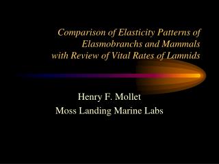
A review of age and growth, reproductive biology, and demography of the white shark, Carcharodon carcharias Henry F. Mollet Moss Landing Marine Labs
http://homepage.mac.com/mollet/Cc/Cc_litters.html Med Sea Summer 1934 Taiwan Oct 1997 Japan Feb 1985
Update: White shark litter of 8;50-60 cm TLTaiwan 13 October 1997 (Victor Lin p.c.)
5.55 m TL Kin(-Town) white shark caught on 16 Feb 1985 • Uchida et al. (1987, 1996) assumed near-term embryos were aborted. • 192 eggcases of 3 types (66 + 20 + 101; 104, 33, and 14 g) weighing 9 kg in left uterus. • Early-term more likely (Mollet et al. 2000). • No blastodisc eggcases? Overlooked? How old?66 - 192 days?
Shortfin mako 3 cm TL embryos.How old? • 4(L) +5(R) blastodisceggcases (3x10 cm) with 1 embryo each • > 40 (3x5 cm) eggcases in each uterus with 16-20 eggs per capsule; plus empty eggcases produced before blastodisceggcases • Shell gland produces one eggcase/day (Gilmore 1993 for sandtiger) • Suggested age is 40-50 days (Mollet et al. 2000)
VBGF for 11 embryos and 20 free-swimmersL0 = - 0.060 m; L= 1.837 m; k = 0.977 yr-1; r2 = 0.873
Gompertz for 11 embryos and 20 free-swimmersL0 = 0.027 m; L= 1.513 m; k = 2.649 yr-1; r2 = 0.891
Comparison of VBGF and Gompertz for 11 embryos and 20 free-swimmers
von Bertalanffy (1938) • dM/dt = M2/3 - M, differential equationeta and kappa are anabolic catabolic parameters but no physiological interpretation needed • Substitution method y = M1/3:dy/dt = /3 - /3y; ( = 3k will be used later) • Separation of variable: dy/(/3 - /3y) = dt • Integration: -3/ ln(/3 - /3y ) = t + constant*Constant to be determined by value of y at t = 0* • Final result: y = / - (/ - yo) e-(x/3) t • Back-substitution: M(t) = [/ - (/ - w01/3) e-(x/3) t]3[will become L(t) = L - (L - L0) e-k t ]
L0 versus t0 • VBGF using L0 (von B. 1938) can be transformed mathematically to use x-axis intercept instead of y-axis intercept as 3rd parameter:L(t) = L ( e -k (t - to)); t0 = 1/k ln[(L - L0 )/ L]. • The two formulations are mathematically equivalent. • However, L0 has a biological meaning whereas t0 has none. Therefore, unreasonable L0 are easily detected but not unreasonable t0.
1995 Edmonton in the Lion’s Den Slide • von Bertalanffy was at U of Alberta in Edmonton. • I said it in 1995 and now Tampa 2005: von Bertalanffy (1938) did not use t-zero (not in any of his publications). • t-zero was introduced by Beverton (1954) to simplify yield calculations • Came in widespread use after Beverton and Holt (1957) but it is not helpful for interpretation of VBGFs of elasmos with well defined size at birth (L0).
k is a rate constant with units of reciprocal time • Difficult to deal with/understand reciprocal time. • Better to interpret k in terms of half-life (ln2/k) with units of time. • The time it takes to reach fraction x of Lis given by tx = 1/k ln[(L - L0)/L(1- x)]. • Can use x = 0.95 (Ricker 1979) and L0 = 0.2L: t0.95 = longevity = 2.77/k = 4.0 ln2/k (4 half-life). • Could use x = 0.9933 and L0 = 0: t0.9933% = longevity = 5.00/k = 7.21 ln2/k (~ 7.2 half-life, Fabens 1965) • x = 0.95 vs. x = 0.9933 produces large range of longevities that differ by almost a factor of 2! (7.21/4 = 1.80)
L is inversely proportional to k • We started with dM/dt = M2/3 - M • Steady state means dM/dt = M2/3 - M = 0 after a long time when t = i.e. M () = M (L() = L ) • Therefore M1/3= / (L = q (/) will become L=3q (/k)L is inversely proportional to k • The steady state value (final mass or length) is determined by both and k, the time it takes to get there is determined by k only.
Various 2-parameter VBGF’s • 2-parameter VBGF (using size at age data) by using observed size at birth for L0. Justification: If one had age versus length data for neonates that’s what the data would have to be. • Fabens for tag-recapture data, also a 2-parameter VBGF (k and L). Length at tagging and recapture and time-at-large data are used. • Gulland-Holt, yet another 2-parameter VBGF (k and L) which is usually used in graphical form by plottingannualized growth versus average size.
Observed # of band-pairs in 3 populations. White sharks in SA appear to be younger for given TL?
Maximum band count/age?Might be 30- 40 yearsWill show later (2nd talk) that longevity () is important • Gans Baai 23 bands, CD not available? TL ~ 5.6-6 m (Dave Ebert, Mollet et al. 1996). • North Cape, 22+-1 bands, CD 63 mm only but not max size. TL ~ 5.36 m; (bands were stained by mud, disappeared in air) (Francis 1996). • Cojimar Cuba 1945 6.4 m TL? specimen had 80x37 mm vertebrae, no band counts given. • Taiwan ~5.6 m TL specimen had 83x36 mm vertebrae, 16-22 bands (Sabine Wintner).
VBGF and Gompertz for combined data from around the world (mostly juvenile white sharks) n = 185 VBGF GompLo 1.5 1.6 mLoo 6.2 5.5 mk 0.079 0.144 y-1t95% 35 22 y
Combining embryonic and post-natal data. Embryonic growth is expected to be larger than post-natal growth; cannot use same growth function n = 216 VBGF GompLo 1.45 1.49 mLoo 5.92 5.2 mk 0.088 0.17 yr-1t95% 31 19 yrt-zero -3.2 - yr
Embryonic and wild vs. captive 1st year growth • Assume gestation period of 1.5 yr, growth will be 1.3-1.5/1.5 = 0.81 - 1.0 m/yr. • Calculated 1st year growth from existing VBGF’s much smaller at 0.25-0.35 m/yr • However, captive growth at MBA with feeding to satiation was 0.8 m/yr. • Female would mature in 5 instead of 15 yr? • Captive neonate pelagic stingrays (male and female) may have reached maturity within 1 year!
Preparation for Elasticity talk:Vital rates for white shark • Age at first and last reproduction: = 15 yr, = 60 yr; / = 4.0; Mollet and Cailliet (2002) but 45 yr; / 3.0. • Annualized female fertility m = 8.9/2*3 = 1.4833; • Mortality = - ln(0.01)/60 = 0.07675S = exp(-M) = 0.9261; • Discounted fertilities Fi = m .Si = 1.3737(same for pre- and post-breeding census because survival to age 1 (S1) was assumed to be same as juvenile and adult survival).
Elasticity matrix for white sharkE-pattern comprising E(m), E(js), and E(as)can be obtained by summing over appropriate matrix elements but need to include discount
Results: 1 = 1.082, (r1 = ln(1) = 0.07869); Abar = 20.91 yr (Abar/ = 1.394), T = 23.11 yr, 1 = 26.15 yr. E-pattern: E(m) = 0.04564 E(Sj) = 0.6846, E(Sa) = 0.2697 (E(Sa)/ E(Sj) = 0.394).
Summary Slide • We know very little about details of reproductive biology of white shark. • The good news is that we know enough. • We can formulate management proposals using prospective elasticity analysis with available inadequate data. • Thanks to Sabine Wintner and Barry Bruce for sharing raw vertebrae count data.
Recipe for management proposals based on E-pattern from prospective elasticity analysis(To be proved in afternoon presentation) • Use E-triangle to graph E-pattern comprising elasticities of fertility, juvenile survival, and adult survival. E1 = E(m), E2 = E(Sj), E3 = E(Sa). • E-pattern is determined by and Abar alone(don’t even need E-matrix). • Most important is ratio E3/E2 = Abar/ - 1.If / 3.0 then E3/E2 3.0 without further considerations (most elasmos). • E2/E1= (obviously large means that E2 >> E1) • One complication, if repro cycle is not 1 yr. White shark as example: E2/E1 = = 15 yr say. If repro cycle is 3 yr then E2/E1 = = 15/3 = 5 (3-yr units). E3/E2 stays about the same!