
Volume Rendering & Shear-Warp Factorization
Volume Rendering & Shear-Warp Factorization. Joe Zadeh January 22, 2002 CS395 - Advanced Graphics. Volume Rendering (Part II). 3D Radiology Lab, Stanford. Start with Slices (usually). Stanford. Classification. What does this voxel represent? Classification via probability

Volume Rendering & Shear-Warp Factorization
E N D
Presentation Transcript
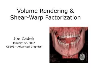
Volume Rendering & Shear-Warp Factorization Joe Zadeh January 22, 2002 CS395 - Advanced Graphics
Start with Slices (usually) Stanford
Classification • What does this voxel represent? • Classification via probability • Assign (R,G,B,) • Create Isosurfaces
Marching Cubes Lorensen and Cline
Watt, pg 385 OBJECT IMAGE
Image Order: Ray Casting • Cast set of parallel rays • Remain Traveling • Two Issues • Find voxels through which the ray passes • Find a value for the voxel NOT RAYTRACING!!!
Watt, pg 386 Image Order: Casting Image
Watt, pg 387 Image Order: Compositing with Resampling
Watt, pg 388 Image Order: Resampling (Shear) then Compositing
Object Order: Voxel Projection • Splatting
The Paper • “Fast Volume Rendering Using a Shear-Warp Factorization of the Viewing Transform” • SIGGRAPH ‘94
The Authors • Philippe Lacroute • Computer Systems Laboratory, Stanford • PhD Dissertation with same title • SGI for 3 years • Marc Levoy • Computer Science Dept, Stanford • 1996 SIGGRAPH Achievement Award for Volume Rendering
History of the Stanford Bunny O’Brien, Hodgins: “Animating Fracture”
Image Order vs. Object Order • Image Order (ray-casting) • Redundant Traversals of Spatial Data • Early Ray Termination • Object Order (splatting) • Traverse through complete spatial data • Only Traverse Once
The Shear-Warp Revolution • Takes the good of both Object and Image Order Algorithms
3 Steps • “Factorization of the viewing matrix into a 3D shear parallel to the slices of volume data” • “a projection to form a distorted intermediate image” • “and a 2D warp to produce the final image”
In a Nutshell • Shear (3D) • Project (3D 2D) • Unwarp (2D)
The Shear (Parallel) Lacroute, Levoy
The Shear (Perspective) Lacroute, Levoy
Sheared Object Space • Intermediate Coordinate System • Simple mapping from object oriented system • All viewing rays are parallel to the third axis
Properties of Sheared Object Space • Pixel scanlines of intermediate are parallel to voxel scanlines • All voxels in a slice scaled by same factor. • (Parallel) Every voxel slice has same scale factor (voxelpixel is one-to-one)
Algorithm, again • Transform volume to sheared object space by translation and resampling • Project volume into 2D intermediate image in sheared object space • Composite resampled slices front-to-back • Transform intermediate image to image space using 2D warping
Three Shear-Warp Algorithms • Parallel Projection • Perspective Projection • Fast Classification • (SW Parallel Projection first described by Cameron and Undrill, 1992)
Parallel Projection Rendering • Recall: Voxel scanlines in sheared volume are aligned with Pixel scanlines in intermediate • Both can be traversed in scanline order • Simultaneously
Compress Voxel Scanlines • Run-length encoding • Skip transparent voxels RTAAAASDEEEEE = RT*4A SD*5E • Effectiveness depends heavily on image type
Compress Intermediate Image • Recall: Splatting doesn’t account for occlusion • Solution: Keep run-length encoding of opacity while creating the intermediate image • If a pixel exceeds an opacity threshold, we know we don’t have to go to deeper slices (I.e. ray termination)
For the Uncompressed • Recall: All voxels in a given slice are scaled by the same factor • Other rendering algorithms require a different scaling weight for each voxel • Use Bilinear Interpolation and backward projection • Two voxel scanlines single intermediate scanline
Warping • We now have composited intermediate image • Warp: Affine image warper with bilinear filter • We now have our image
Some Costs • Run-length encoded volume • Preprocessing created • View Independent • Three encodings (x,y,z) • Still less data than original volume because omits transparency
256x256x225 on SGI Indigo R4000 Lacroute, Levoy
Perspective Projection • Majority of Volume Rendering Parallel (’94) • Perspective mostly useful in radiation beam planning • Viewing rays diverge, complicating sampling
Perspective Projection Algorithm • Almost exactly like Parallel • In addition to translation during shear, scale as well; then composite. • Tends to create a many-to-one mapping from voxels to pixels • Slower in calculating: volumes and intermediate scanlines not traversed at same rate
Fast Classification Algorithm • Recall: Previous two algorithms require intense preprocessing classification step • Not acceptable when experimenting with different opacities • Solution: Classification opacity via scalar function
The Algorithm Lacroute, Levoy
A bit more detail • For some block of volume, find extrema of parameters to opacity function • If function returns transparent opacity, discard scanline portion • Subdivide scanline and repeat recursively until size of portion is smaller than a threshold
Further Analysis • 1283: 5x speed increase over traditional ray-casting (.5 sec) • 2563: 10x speed increase (1 sec) • General Shear-Warp: O(n) • Classification with Render: O(n2)
Pitfalls of Shear-Warp • Two resampling steps • No noticable degradation • Uses 2D reconstruction filter to resample the volume data • Not really applicable
Futher Research • Algorithm is parallelizable • Real-Time Rendering on Shared Multiprocessors (approx 10 fps) [SGI Challenge 16 Processor multiprocessor, 256x256x223 voxel] • Volpack