Multi-tier Data Access and Hierarchical Memory Design: Performance Modeling and Analysis
470 likes | 627 Views
Multi-tier Data Access and Hierarchical Memory Design: Performance Modeling and Analysis. Marwan Sleiman PHD Defense Department of Computer Science & Engineering University of Connecticut 371 Fairfield Road Unit 2155 Storrs, CT 06269 Major advisor: Dr. Lester Lipsky Associate advisors:

Multi-tier Data Access and Hierarchical Memory Design: Performance Modeling and Analysis
E N D
Presentation Transcript
Multi-tier Data Access and Hierarchical Memory Design: Performance Modeling and Analysis Marwan Sleiman PHD Defense Department of Computer Science & Engineering University of Connecticut 371 Fairfield Road Unit 2155 Storrs, CT 06269 Major advisor: Dr. Lester Lipsky Associate advisors: Dr. Reda Ammar Dr. Swapna Gokhale Dr. Chun-Hsi Huang
Overview of the Presentation • Introduction & previous work • Motivation and Objectives • Markov-Chain model and performance metrics • Interdependence of the hit ratios between the levels • Design Constraints • Approximation Function • Power-Tailed aspect of the memory access • Effect of increasing the cost on performance • Improving the performance while maintaining a constant cost • Optimization techniques • Performance measures • Conclusion and Future work
Hierarchy of Storage Systems • Storage systems are present in several forms and on different hierarchical levels; they expand the concept of the classical hierarchy beyond the local machine: • Registers, caches, main memory (RAM), disks, tapes, middle-tiers, network storage, internet storage. • Storage systems provide the basic functions of : • storing data permanently • holding data until it is accessed and processed
CPU Access Time Level 1 X1 Xi Level i Level n Xn XM M Hierarchical Memory Model
Storage Systems and Performance • Fast memory access is vital to achieving superior system performance • Because of the gap between the CPU speed and memory access time, • memory access time is increasingly becoming bottleneck to system performance • Thus the applications cannot benefit from a processor clock-speed upgrade • Speed is expensive! => $$ cost must be optimized
Solution • Increasing the speed and size of the existing levels. • Inserting smaller and faster intermediate memory levels • Which one is better? * We need to evaluate the cost and performance of each alternative
Previous Work • Du et. al. ’00 showed the importance of the depth of the memory hierarchy as a primary factor on a cluster of workstations but their results are dependent on the workload type. • D. G. Dolgikh et al ‘01 show the importance of developing an analytical model to optimize the use of web cashes. • Jin et al. ’02 developed a limited analytical model that captures only a two-level cache, but we see in their work a big discrepancy between the predicted and measured memory performance. • El-Zanfaly et. Al ’04 presented an analytical model to study the performance of Multi-Level cashes in Distributed Database Systems. • Garcia Molina and Rege ‘76 and Nagi ‘06 demonstrated that, in some cases, it is more suitable to use a slower CPU for effective utilization of memory. • E. Robinson and G. Cooperman ‘06 showed that, in certain conditions, it can be more efficient to discard the memory and use a disk-based architecture than using the memory –which means reducing the memory hierarchy.
Motivation • Memory hierarchy is becoming more complex. • Memory access time differs from application to application • The average memory access time is a crucial factor in system performance, also other performance metrics and measures may be important and must be taken into consideration. • Despite having small mean time for certain cases, for an infinite hierarchy, the time may have unbounded higher jthmoments E[|T- Tavg |j]= => Long queues of memory accesses and hence can take quite some time draining them out while affecting system performance severely (pipelined processors & shared memory cases) • It is necessary to develop a universal model able to cover all possible cases.
Our Objectives: Several objective functions help us improve the performance of hierarchical memory systems: • Minimizing the mean memory access time. • Minimizing the memory queueing time for a given arrival rate by using the P-K formula for an M/G/1 Queue. • Minimizing the probability of exceeding a long delay time • Do these objectives have the same optima? If not, what about a Trade-off? What is (are) the best optimization technique(s)? Proposed an approximation to the above functions by maximizing the ratio of time lag to variance for a given objective time to minimize the width of the confidence interval and reduce the probability of exceeding the target time.
1- h1 XLi 1-h(n-1) XLn 1-h(i-1) 1-hi XL1 Li Ln 1-hn L1 1 hi hn M S0 h1 1 1 Dn D1 Di 1 1 1 1 XD1 XDi XDn State Transition Diagram
Notation • n is the depth of the memory hierarchy, L=n+1 is the total number of memory levels • P is the sub-stochastic matrix that corresponds to the transitions from one state to another one. Its dimension is (2n+1)*(2n+1) • p is the entrance vector that corresponds to the state of the system at the first memory request. p is a row vector of size 2n+1, where n is the number of intermediate levels. p=[1 0 0 ….0] • is the unit column vector of size 2n+1. • M is the transition rate matrix; it corresponds to the rates of leaving the state. M is a diagonal matrix of dimension (2n+1)*(2n+1). • I is the identity matrix of the same dimension as P and M. • h is the hit ratio, ĥ =1-h.
Sub-stochastic Matrices B = M(I –P)and V = B-1.
Access Time Calculations Let X be the random variable denoting the memory access time. • Assuming we have memories with exponential service times, the pdf of the ith memory level is given by: • The jth moment of the access time is given by: • The mean access time is given by the first moment and does not depend on whether the memory service time is exponential or not. • The variance of the access time is given by:
Non Exponential Memories • Each node is represented by the vector-matrix pair: <pi,Bi> its pdf is: • The mean access time remains the same. • However the variance differs by a correction term compared to the exponential case e: Cvi2 is the coefficient of variation of the non-exponential stage i. For Exponential memories, *This is an innovation! (CATA 2006)
More performance metrics Let Ty be the random variable denoting the mean system time. • The Pollaczek-Khintchine formula (called P-K formula) is used to calculate the mean waiting time spent by a customer in an M/G/1 Queue: • Where, is coefficient of variation, is the utilization factor, is the arrival rate. • The probability of exceeding a long delay time, Pr(X>z), is given by the reliability function for our hierarchical memory system:
Interdependence of the Hit Ratios Let Y be the Random Variable representing the data fetched in memory and Mi the dataset in memory level i, MiMi+1. We define the following additional terms: the probability of finding data in the intermediate memory level i the size of memory level i. the cost per unit of size of each memory level i. We assume that: , where is a constant; The total cost of the L-level hierarchical system becomes:
Interdependence of the Hit Ratios (continued) is the local hit ratio at memory level i,
Design Constraints If we consider any L-level hierarchical memory with total cost C, there are constraints on the sizes of the levels we can select: For simplicity of calculations, we assume in what follows that the memory access time increases geometrically from one level to the next and the cost decreases geometrically:
Power-tailed Aspect of the Memory Access Time • A power-Tailed (also called Pareto Distribution) function with parameter is a function that has infinite high moments. • Its reliability function, • We showed that, if we have the same hit ratio, h, at all levels, the moments become unbounded as the number of hierarchies goes to infinity: For (1-h) j 1, iff where,
Simulations • Three plots for the reliability function with power tails obtained by simulating 100, 000 memory accesses • The system has 10 memory levels with hit-ratios h = 0.3, 0.5 and 0.7 with µ = 1, =1 and = 2 • The slopes of the plots are equivalent to the slopes ( > 0) in the reliability function for the power-tailed distribution:
Log R(z) vs Log(z) plot shows power-tailed aspect of access time
Two-Level Cache Memory 1- h1 XL2 XL1 L2 L1 1-h2 1 M S0 h2 h1 1 1 D1 D2 1 XD2 XD1
Effect of doubling the Cost on Exponential & Non-Exponential Memories in a 2-level cache memory Plots of the mean and variance for exponential and non-exponential 2-level memory hierarchies versus the size of the outer memory. The lines correspond to the original system and the dashes correspond to a system with double cost. The non-exponential has a gamma of 4.
Behavior of the Hit Ratios in a 2-Level Cache Memory. Behavior of the memory hit ratios as we change the size of the lower/outer memory level and increase the cost of the memory system. A level may become obsolete because it has a low hit ratio.
Queueing Time vs Access Time Mean memory access time E(X) and mean queuing time E(Tl) versus the size S of the Outer-level memory in a 2-Level hierarchical memory system. E(X) has its minimum for S = 71, while E(Tl) has different minima depending on the value of l. There is a difference of 8 % between Min[E(T)] and its value at Min[E(X)] for the same outer memory size! This difference increases as the arrival rate increases.
Inserting an Upper Faster Level XL2 XL1 1- h1 XL0 1- h0 C1 C2 1-h2 1 C0 Cm h1 a1 h2 S0 a2 h0 a0 XD0 XD1 XD2 D0 1 D1 1 D2 1
Increasing the Size vs Inserting Intermediate Levels Increasing the size of the exiting levels versus inserting intermediate memory levels.
Exceeding a Long Delay Time The probability of exceeding a long delay time is given by the reliability of our hierarchical memory system: Plots of the mean, variance and reliability function for exponential 2-level and 3-level memory hierarchies versus the size of the outer memory. The straight lines correspond to 2-level memory systems and the dotted lines correspond to 3-level memory system. The mean is plotted in blue and the probability of exceeding a target time is plotted in green.
Effect of the memory levels on the probability of exceeding a long delay time Effect of the memory levels on the probability of exceeding a long delay time on a log scale: The curve of the reliability is steeper when the system includes an upper level memory system. E(X)= 4.78 for the 3-level memory, E(X)=6.91 for the 2-level memory with the upper level removed, and E(X)=5.81 for the 2-level memory with the upper level removed.
Probability of Exceeding a Long Delay (continued) Probability of exceeding a long delay time for 2-Level and 3-Level hierarchical memories on a log scale: As the access time becomes greater than 100ns, the reliability curves become tangent to their asymptotes. E(X)= 4.78 for the 3-level memory, and E(X)=6.91 for the 2-level memory.
Exceeding a Long Delay Time: Asymptotic Behavior • From the spectral decomposition theorem, R(z) is given by: (1) • Where: is the ith Eigenvalue of the matrix B is the ith column Eigenvector of the matrix B, that is is the ith row Eigenvector of the matrix B, that is • The probability of getting memory requests that take a relatively long time along this stochastic hierarchy is given by finding the limit of R(z) as z becomes very high and it is dominated by the mth term of R(z) having the smallest Eigen-Value. • Let thus , and (2) • So if we plot the probability of exceeding time x on a semi-log scale, we find out that it approaches the curve: that intercepts the y-axis on a semi-log graph at the value
Exceeding a Long Delay Time 3-D • 3-D plot of the probability of exceeding a Long Delay Time R(z) for a three-level memory versus the size of the intermediate memory levels: Sb is the index of the upper memory level and Sc is the index of the lower level. We remark here that the curve of R(z) is steeper with respect to the upper level growth because R(z) is more sensitive to it, however it is more flat with respect to the lower level because it is less sensitive to it.
Optimization techniques • Local search • Lagrange Multipliers Method We assume that:
Analytic Solution for Minimizing E(X) Optimizing E(X) versus the total cost: • Because our model is a Feed-forward Network, the total access time for this memory system is given as a function of the intermediate memory sizes by: • So we have to optimize subject to the following total cost constraint: • By using Lagrange Multipliers method, we will have:
Lagrange Multipliers method and constant hit ratios • By solving these equations, we get:
Plot of the hit ratios at steady state (PT) Hit Ratios versus cost for a three-Level Hierarchical memory: h2 and h3converge to a constant determined by
Difference between E(X) and E(Tl) for a 3-level hierarchy Mean memory access time E(X) and mean queuing time E(Tl) versus the total memory cost for a 3-Level Hierarchical memory. The difference between the minimal queueing time and the value of queueing time at the optimal mean memory time is more significant here and is of the order of 15%.
Difference between E(x) and E(Tl) for a 3-level hierarchy Optimal system time, Min[E(Tl)] versus the value of E(Tl) at the optimal mean system time, E(X), versus the total memory cost for a 3-Level Hierarchical memory. The relative difference between the minimal queueing time and the value of queueing time at the optimal mean memory time decreases as we decrease the cost.
CPU L1 L2 m CPU CPU CPU L1 L1 L2 L2 L3 L3 L3 m m m System 1 System 2 System 3 System 4 Performance Measures Different hierarchical memory architectures with intermediate levels at different locations: The closer the memory is to the CPU, the smaller and faster it is.
Observations • Observation 1: for the same cost, inserting an intermediate memory at the upper level results in a system with a lower mean time. • Observation 2: for the same cost, inserting an intermediate memory at the upper level results in a system with a smaller probability of exceeding a small delay time and higher probability of exceeding a high delay time. • Observation 3: for the same cost, inserting an intermediate memory at the upper level results in a system with a worse variance regardless of the distribution of the service time of the intermediate memory levels. • Observation 4: a higher variance corresponds to a lower hit ratio at the upper memory levels. • Observation 5: the variance of the memory access time is relatively high. Such a high variance can dramatically affect the performance of some architectures sensitive to a high access time such as pipelined, decoupled, and multi-grid architectures. So it is important to consider optimizing the variance of hierarchical storage. • Observation 6: doubling the cost of the hierarchical memory has a positive effect on all the performance metrics but in different ratios. Each of the performance metrics improves in a different way than the others to the modification of the memory architecture (number of levels, size, cost, etc…) because these performance metrics have different optimal points. • Observation 7: the probability of exceeding a target time is more sensitive to the upper memory level than the lower level and it improves at a faster rate by optimizing the upper level size than by optimizing the lower levels. • Observation 8: if cost and speed are proportional (i.e. there is a geometric relationship between the levels), we get an optimal access time when we have CiSi= Ci+1Si+1that is when we invest the same in each level. • Observation 9: there is a linear relationship between the probability of going to the main memory, Pm, and the value of am in equation 2. We have found that the ratio is a constant:
Conclusions • Markov-Chains can model the access time of hierarchical memories. • Our analytical model is very powerful and universal and very flexible. • The hierarchical memory access can be power-tailed. • The variance is not the same for non-exponential memory stages. • The different performance metrics don’t have the same optima => designing an optimal system is application dependent.
Contributions • Robust Analytical Model (Independent of the application, number of levels and architecture) • New performance Metrics • Effect of location and proximity of the Memory Levels • Power tailed aspect of the memory access
Future Work • Running more simulations to validate our model and make sure it is realistic and reflects the real computing environment. • Using memory profiling-related tools (PurifyPlus, Valgrind, Insure, VTune) • Including models that account for localities and working sets. • Studying the sensitivity to each performance metric and finding its effect on performance. • Trying different architectures (like decoupled architecture, dual-processor and shared memory). • Studying memory hierarchies with more levels. • More optimization techniques like NN.
Publications • “Moments of Memory Access Time for Systems with Hierarchical Memories,” 21st International Conference on Computers and Their Applications (CATA-2006), Seattle WA, March 2006. With Lester Lipsky and Kishori Konwar. • “Performance Modeling of Hierarchical Memories,” 19th international conference on computer applications in industry and engineering (CAINE-2006), Las Vegas, Nevada USA, November 13-15, 2006. With Lester Lipsky and Kishori Konwar. • “Multi-channel Software-Oriented Pulse Width Modulation (SPWM),”21st International Conference on Computers and Their Applications (CATA-2006), Seattle WA, March 2006. • “Dynamic Resource Allocation of Computer Clusters with Probabilistic Workloads,” Marwan Sleiman, Lester Lipsky, and Robert Sheahan in the proceedings of the 20th IEE International Parallel & Distributed Processing Symposium, April 25-29 Rhodes Island, Greece. • “Multi-Tier Data Access & Hierarchical Memory Optimization,” submitted to the 20th International Conference on Parallel and Distributed Computing Systems. With Lester Lipsky. • “Moments and Distributions of Response Time for Systems with Hierarchical Memories,” submitted to the International Journal of computers and Their Applications. • “Performance Metrics of Hierarchical Memories,” to be submitted to the International Journal of computers and Their Applications.
The End Questions & Suggestion? marwan@engr.uconn.edu Thank You!