Download
1 / 31
320 likes | 458 Views
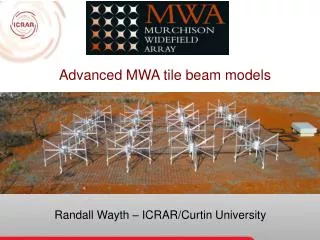
Advanced MWA tile beam models . Randall Wayth – ICRAR/Curtin University. MWA Primary beam. Team: Adrian Sutinjo , John O’Sullivan, Emil Lenc , Shantanu Padhi , Tim Colegate , Budi Juswardy , RW. Background: Beam amplitude bootstrapping in MWA GLEAM Survey

E N D
Advanced MWA tile beam models Randall Wayth – ICRAR/Curtin University
MWA Primary beam Team: Adrian Sutinjo, John O’Sullivan, Emil Lenc, ShantanuPadhi, Tim Colegate, Budi Juswardy, RW • Background: • Beam amplitude bootstrapping in MWA GLEAM Survey • “False Q” seem by Emil in high freq, large zenith angle obs • Q/I = (XX-YY)/(XX+YY) • Cal solutions transferred from calibrator close to zenith. • Current model of tile is analytic: = array factor * dipole pattern. No mutual coupling.
GLEAM background • Meridian drift scans • Night-time observing • 8-10 hours of RA per campaign • Week-long campaigns • 7 DECS, 1 DEC per night, all freqs 80-230 MHz • Year 1: • GLEAM 1.1: Aug 2013 (RA 19 – 3 ) • GLEAM 1.2: Nov 2013 (RA 0 – 8 ) • GLEAM 1.3,1.4: 2014-A (6-16, 12-22)
GLEAM 1: 2013/14 6 h 12 h 0 h 18 h 12 h +90 0 -90 GLEAM 1.3 Feb 2014 GLEAM 1.2 Nov 2013 GLEAM 1.1 Aug 2013 GLEAM 1.4 May 2014
GLEAM 1: 2013/14 As at Dec 2013 6 h 12 h 0 h 18 h +90 0 Complete! -90 GLEAM 1.3 Mar 2014 GLEAM 1.2 Nov 2013 GLEAM 1.1 Aug 2013 GLEAM 1.4 May 2014
MWA Primary beams • Background: when calibration sol’n from 3C444 (DEC-17) are transferred to the DEC -27, -14, and 1.6 scans at 216MHz • Clearly the magnitude of XX and YY are off. (phase OK)
Fitting a simple primary beam model Based on work @189MHz in Bernardi et al, 2013.
Inter-port (mutual) coupling model Known (=LNA impedance, diagonal) Known (=delays) Unknown (=dipole complex ‘gain’) Known (=impedance matrix, via sims)
Example Z_tot matrix, 216MHz NS-NS interactions EW-EW interactions NS-EW interactions
How about other freqs? 186 MHz No gradient across tile Modest gradient across tile
How about other freqs? 155 MHz No gradient across tile No gradient across tile
What’s going on? • Dipole is 74cm across = ½ wavelength at ~200 MHz • Below this freq, short dipole approximation is increasingly valid • Also, magnitude of coupling decreases with freq
What’s going on? • The phase delay gradient forces “side-to-side” interactions on the “X” bow-ties as opposed to “end-to-end” interactions on the “Y” bow-ties. • Such asymmetry does not occur when pointing the telescope in the diagonal plane as the interactions are symmetric with respect to the “X” and “Y” bow-ties. • “end-to-end” vs “side-to-side” asymmetry is reduced with increasing wavelength. Direction of increasing delay for az=0, za > 0
The way forward • Three tier model: • Analytic dipole model with impedance matrix from simulations or measurements • (basically what has been presented in this talk) • Average dipole response based on simulations with impedance matrix. One lookup pattern per freq. • Relatively straightforward • Individual dipole pattern for each dipole per pointing per frequency. • Expensive
How well can we do with 2nd tier? 216 MHz, ZA=14 deg Blue line: predicted false Q for simple model using incorrect (old) model for calibration Red line: expected false Q for 2nd tier model using 3rd tier model as “truth”. (zero is good)
How well can we do with 2nd tier? 155 MHz, ZA=14 deg Blue line: predicted false Q for simple model using incorrect (old) model for calibration Red line: expected false Q for 2nd tier model using 3rd tier model as “truth”. (zero is good)
Tile: bottom line • Mutual coupling does affect the tile beam, especially at higher freqs (>= 200 MHz) • At high freqs, far from zenith along cardinal axes (0,90 degsaz) mag and phase is quite different • Cal solutions for amplitude are only valid at that pointing (this is not new, but model is…) • “False Q” due to transferring near-zenith amp cal to off-zenith meridian data. • Mutual coupling also affects the relative response of dipoles, even at the zenith. This can taper the tile response, hence affect beam width and sidelobes.
Optical H-alpha image: Luigi Fontana. http://www.astrobin.com/27523/B/
Rosette Nebula Barnard’s loop Orion Nebula Optical H-alpha image: Luigi Fontana. http://www.astrobin.com/27523/B/
Impedance matrix: 32x32 Labels: 1-16 N-S “Y” dipoles 17-32 E-W “X” dipoles