Download
1 / 39
390 likes | 678 Views
ML Estimation of the General Error Variance and Nonlinear Models. ML Estimation of Linear Models with General Covariance Matrix. Lets return to our general model where: y=X β + e y is a (T x 1) vector of obs. on the dependent variable

E N D
ML Estimation of the General Error Variance and Nonlinear Models
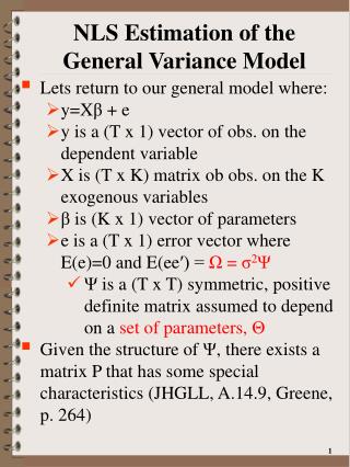
ML Estimation of Linear Models with General Covariance Matrix • Lets return to our general model where: • y=Xβ + e • y is a (T x 1) vector of obs. on the dependent variable • X is (T x K) matrix of obs. on the K exogenous variables • β is (K x 1) vector of parameters • e is a (T x 1) error vector where E(e)=0 and E(ee′) = Φ = σ2Ψ • Ψ is a (T x T) matrix assumed to depend on parameters Θ, Ψ = Ψ(Θ) • Dimension of Θ and how Ψ depends on Θ is a function of assumptions made about the data generating process (e.g., heteroscedasticy vs. autocorrelation) scaler
ML Estimation of Linear Models with General Covariance Matrix • Previously, we developed a number of 2-step estimators depending on the structure of Ψ: • AR(1) • Multiplicative Heterscedasticity • In these 2-step approaches • Θ are estimated from information provided by the CRM residuals • Ψ(Θ) developed using above estimates • FGLS procedures used • As an alternative, lets see how we can use ML techniques to estimate the parameters of the general linear model directly
ML Estimation of Linear Models with General Covariance Matrix • If we assume that the error term and therefore y are both normally distributed, the total sample log likelihood function for (β,Θ) can be written as: Exogenous variables Φ(Θ*) = σ2Ψ(Θ) Θ* = σ2|Θ
ML Estimation of Linear Models with General Covariance Matrix • Similar to the CRM we saw earlier that maximization of L with respect to β and σ2 conditional on Θ results in • If we substitute the above definition of βG into the original likelihood function • We obtain the concentrated log-likelihood function • Only a function of exogenous data and Θ, the parameters of the error covariance matrix βG does not depend on σ2
ML Estimation of Linear Models with General Covariance Matrix • This implies the concentrated log-likelihood apart from constants is: eG = y – XβG(Θ)
ML Estimation of Linear Models with General Covariance Matrix • The maximum likelihood estimator for Θ, ΘL is that value of Θ for which L*(Θ) is a maximum • Given the concentrated log likelihood: • Lets define a modified weighted sums of squared errors, S*(Θ)
ML Estimation of Linear Models with General Covariance Matrix • Given the above positive monotonic transformations, the value of Θ that maximizes the concentrated log-likelihood function is also the value of Θ that minimizes S*(Θ) • The presence of the term |Ψ(Θ)|1/T differs from our previous definition of the weighted sum of squared errors under the general variance model, • S(β,Θ)=e′GΨ(Θ)-1eG S*(β,Θ)= e′GΨ(Θ)-1eG|Ψ(Θ)|1/T • If Ψ(Θ) does not depend on T, as T→∞, |Ψ(Θ)|1/T →1 which implies S*(β,Θ)→ S(β,Θ)
Maximum Likelihood and Mult. Heteroscedasticy Linear wrt β Nonlinear wrt α • Lets return to our multiplicative heteroscedasticy example we set up before where: • Yt=Xtβ + et E(e2t) = σ2t=exp(Wtα) =σ2exp(W*tα*) Wt=(1,W*t) t=(1,…,T) α' = (ln(σ2) α*) • Φ is a diagonal matrix w/tth diagonal element: σ2t=exp(Wtα) • JHGLL, p.538-541, 548-551, Greene, p.522-527
Maximum Likelihood and Mult. Heteroscedasticy • If we assume the error terms follow a multivariate normal distribution then the sample log-likelihood is: σ2=exp(α1)
Maximum Likelihood and Mult. Heteroscedasticy • Under this framework, the information matrix can be derived: S = # of variance exog. variables Assumed normal distribution For β’s W is TxS vector of exogenous data For α’s vs. 4.9348(W′W)-1 under 2-step method
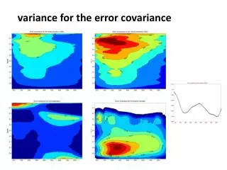
Maximum Likelihood and Mult. Heteroscedasticy ML Model of Multiplicative Hetero. Proc Defining Likelihood Function Dep. & Exog. Variables Numerical Gradients Maximum Likelihood Procedure Estimates of , Starting Values Proc for Calc. Variances ,
Maximum Likelihood and Mult. Heteroscedasticy • ML estimation of multiplicative heteroscedasticity model • JHGLL, pg. 538-541, Table 9.1 • MATLAB Code uses the BHHH algorithm • I use the 2-step results as starting values for the ML estimation (K x 1) step BHHH Lt is tth contribution (K x K)
Maximum Likelihood and Mult. Heteroscedasticy • ML estimation of multiplicative heteroscedasticity model • MATLAB Code: • ∂L/∂θ = Z, use numerical gradients • H = Z′Z Pn= -solve(H) • db = (solve(H)%*%colSums (z)) • Overview of Results Analytical Gradients LLF Function full step R commands H
Maximum Likelihood and Mult. Heteroscedasticy • I use two methods to obtain parameter covariance matrix: • BHHH method (Numerical) • -Pn • Previous Analytical Analytical Gradient Function 15
Maximum Likelihood and Mult. Heteroscedasticy • As an alternative to the BHHH algorithm used in the above MATLAB code • I(Θ) is block diagonal (given the functional form of the heteroscedasticity) • Judge et al., p.540., recommend using the method of scoring (GN) to undertake the iterations separately for β and α .
Maximum Likelihood and Mult. Heteroscedasticy • That is, for β under the method of scoring we have: • Given the above structure of the Hessian matrix, one can show that
Maximum Likelihood and Mult. Heteroscedasticy • where Wt is a (1 x D) vector of variables on which the variance of et depends and Xt is (1 x K) • Note the dimensions used in the JHGLL discussion and that presented here, there is a difference
Maximum Likelihood and Mult. Heteroscedasticy • Similarly, for α under the method of scoring we have:
Maximum Likelihood and Mult. Heteroscedasticy • Testing for Multiplicative Heteroskedasticity Using 3 Asymptotic Tests • H0: Homoscedasticity H1: Multiplicative Heteroscedasticity • H0: α2=α3=…=αS=0 H1: at least one of the above ≠0 • Continuing with our example (Table 9.1 JHGLL)
Maximum Likelihood and Mult. Heteroscedasticy • Wald Test • 1 element in α* • Remember Σα,ML=2(W′W)-1 • λW=(0.21732)2[(0.00379774)-1]/2 = 6.218 • χ21,.05=3.84→Reject H0 exog. variables est. coeff. (W*′W*)-1 Var(α2)=2*.003798=0.007596
Maximum Likelihood and Mult. Heteroscedasticy • Lagrangian Multiplier Test • Information Matrix=1/2(W′W) • Σα= 2(W′W)-1 • Using the theoretical results shown in the previous handout λLM=4.028>3.84→reject H0 LM= S(0)′I(0)-1S(0)
Maximum Likelihood and Mult. Heteroscedasticy • Likelihood Ratio Test • Using the full likelihood function LU=-61.748 LR=-64.315 λLR=2(-61.748-(-64.315))=5.134 difference in concentrated LLF’s χ21,.05=3.84
Maximum Likelihood and Mult. Heteroscedasticy • Remember that in general: λW > λLR > λLM • In our empirical example: λW = 6.218 λLR = 5.204 λLM=4.028
Maximum Likelihood and the AR(1) Model • Lets examine another example of the general linear model • Lets assume that we have a linear model where the error terms are autocorrelated with an AR(1) error structure • y=Xβ + e • y is a (T x 1) vector of observations on the dependent variable • X is (T x K) matrix of observations on the K exogenous variables • β is (K x 1) vector of parameters • e is a (T x 1) error vector where E(e)=0 and E(ee′)=σ2Ψ • et=ρet-1 + νt • Var(et) = Var(et+i) = Var(et-i) = σe2
Maximum Likelihood and the AR(1) Model • As we derived earlier, the above implies: Constant variance
Maximum Likelihood and the AR(1) Model • The above implies:
Maximum Likelihood and the AR(1) Model • Previously, we noted that under the general model (and assuming normally distributed error terms), the sample log-likelihood function can be represented as: • Under the AR(1) structure, Ψ(Θ) = Ψ(ρ) • In order to obtain ML estimates of β and ρ all we have to do is build the Ψ matrix e*=Pe P′P=Ψ-1
Maximum Likelihood and the AR(1) Model • As an alternative, using the previous results with respect to the use of ML techniques of the general linear model • The ML estimators for β and ρ are those values that minimize • This expression is similar to what we derived under the general linear model except only συ2 (not β and συ2) has been concentrated out e*=Pe P′P=Ψ-1
Maximum Likelihood and the AR(1) Model • We can evaluate the determinant: |AB|=|A| |B| and P′P=Ψ(ρ)-1
Maximum Likelihood and the AR(1) Model • Summarizing the above: • This implies that: • If T is large and |ρ| is not too far away from 1, the effect of the first term in the above will be small 31
Maximum Likelihood and the AR(1) Model • Given we can use the above to find maximum likelihood estimates of β and ρ as Judge et al, p.534 note, it can shown that Information Matrix (K+2) x (K+2) Previous Result
Maximum Likelihood and the AR(1) Model • Following the results we obtain using the FGLS procedures, the asymptotic covariance and variance estimators are:
Maximum Likelihood Under the Nonlinear Model • y = f(X,β)+e e~N(0,σ2IT) • Using general notation we can represent the sample likelihood function as: Error term assumption nonlinear function e'e 34
Maximum Likelihood Under the Nonlinear Model • The sample log-likelihood function is: • It is not, in general, possible to find an analytical expression for the max. like. estimate, βML such that ∂L/∂β=0 • But, ∂L/∂(σ2)=0→σ2ML=S(β)/T 35
Maximum Likelihood Under the Nonlinear Model • Given the above we can generate the concentrated log-likelihood function wrt only β by replacing σ2 with σ2ML σ2ML For a given T 36
Maximum Likelihood Under the Nonlinear Model • βML that maximizes L*(β|y,X) is identical to the nonlinear least square estimator that minimizes S(β) since S(β)>0 • Equivalence only holds for nonlinear models w/the form: Y=f(X,β) + e e~N(0,σ2IT) 37
Maximum Likelihood Under the Nonlinear Model • y = f(X,β)+e e~N(0,σ2Ψ) where Ψ=Ψ(θ) • We can represent the log likelihood function as: a vector of parameters Weighted SSE’s Z=∂f/∂β 38
Maximum Likelihood Under the Nonlinear Model • Given that an estimate of σ2 is: • We substitute this into the above log-likelihood function to generate a concentrate log-likelihood function with respect to σ2. That is: the terms cancel out 39