Download
1 / 12
120 likes | 248 Views
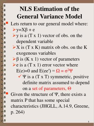
NLS Estimation of the General Variance Model. Lets return to our general model where: y=X β + e y is a (T x 1) vector of obs. on the dependent variable X is (T x K) matrix ob obs. on the K exogenous variables β is (K x 1) vector of parameters

E N D
NLS Estimation of the General Variance Model • Lets return to our general model where: • y=Xβ + e • y is a (T x 1) vector of obs. on the dependent variable • X is (T x K) matrix ob obs. on the K exogenous variables • β is (K x 1) vector of parameters • e is a (T x 1) error vector where E(e)=0 and E(ee′) = Ω = σ2Ψ • Ψ is a (T x T) symmetric, positive definite matrix assumed to depend on a set of parameters, Θ • Given the structure of Ψ, there exists a matrix P that has some special characteristics (JHGLL, A.14.9, Greene, p. 264)
NLS Estimation of the General Variance Model • In general let Ψbeing a symmetric (T x T) positive definite matrix • Matrix P will be a nonsingular (T x T) matrix which will always exist such that: PΨP' =IT → PΨP'(P')-1=IT(P')-1 = (P')-1 → PΨ= (P')-1 → P-1PΨ= P-1(P')-1→ Ψ= P-1(P')-1 → Ψ-1= P'P It Rules of Inverses (AB)-1=B-1A-1
NLS Estimation of the General Variance Model • Given the definition of P, lets redefine the CRM via the following: X*≡PX Y*≡PY e*≡Pe • Y*=X*β + e* →PY=PXβ + Pe P'P=Ψ-1 (TxK) (TxT) (Tx1) (TxT) (Tx1) (TxT) (Tx1) (Tx1) (TxK) Homoscedastic The above are nonlinear function of paramaters given that P=P(Θ)
NLS Estimation of the General Variance Model • 2-step FGLS approaches • Θ estimated from information provided by CRM residuals→ • Ψ(Θ) developed using above estimates • βFG is the value of β that minimizes weighted sums of squared errors conditional on the estimate of error variance structure: • In contrast the NLS estimator for β and Θ, is given by the values of βandΘ that simultaneously minimize S(β,Θ) • Note the difference conditional on
NLS Estimation of the General Variance Model • Remember that P is defined such that P′P=Ψ(Θ)-1 • This implies that P is really P(Θ), a function of Θ • Substituting P(Θ)′ P(Θ) into the above weighted least squares expression E(e*) = 0 E(e*′e*)=σ2IT Functions of Θ
NLS Estimation of the General Variance Model • Given the above, we are concerned with nonlinear least squares estimation of β and Θ in the model: y* = X*β + e* or g(y, X, β, Θ)=e* • The dependence of y* and X* on Θ means that β and Θ enter the above in a nonlinear manner • The above implies that we cannot represent the above as: y = f(X,β, Θ) + e* • The Gauss-Newton and Newton Raphson algorithms we discussed earlier can still be applied to the above general nonlinear model
NLS Estimation of the General Variance Model • If we knew the value of Θ, the estimator of β the minimizes the above weighted sum of squared errors function [S(β,Θ)] is the familiar GLS estimator: • Using this, it is possible to concentrate S(β,Θ) so that it is only a function of Θ • General algorithm for solving this nonlinear least squares problem is to: • Find the value of Θ that minimize S*(Θ), ΘG • Substitute this value into βG(Θ):
NLS Estimation of the AR1 Model • When we reviewed the AR(1) model, I presented a version of the model that could not be estimated either with the CRM or with FGLS given that it was nonlinear in the parameters. • Lets show how NLS could be used to directly estimate this model. • Remember with the AR(1) model we have where νt (t=1,…,T) are iid with mean 0 and constant variance σ2ν
NLS Estimation of the AR1 Model • Alternative estimation method of the AR(1) model: • Y=Xβ+e (t=1,2,…,T) [i] • et=ρet-1+νt → νt = et-ρet-1 • ρyt-1= ρxt-1β + ρet-1 (t=2,3,…,T) • →yt- ρyt-1= xtβ- ρxt-1β +et- ρet-1 • → yt = ρyt-1 + xtβ - ρxt-1β + νt [ii] • Except for omission of the first observation [ii] is the same as [i]. • Error term in [i] is autocorrelated • Error term in [ii] is homoscedastic
NLS Estimation of the AR1 Model • We can modify the above so that the first observation is included: • The weighted sum of squared errors can be represented as: • NLS estimates for β and ρ are those values that jointly minimize S(β, ρ) t = 2,…,T
NLS Estimation of the AR1 Model 11
NLS Estimation of the AR1 Model • We could solve the AR(1) using NLS procedures 12