Apex Point Map for Constant-Time Bounding Plane Approximation
Apex Point Map for Constant-Time Bounding Plane Approximation. Samuli Laine Tero Karras NVIDIA. The Problem. How to quickly find a good bounding plane with a given orientation?. Use Case 1: Ray Tracing and Rigid Motion.

Apex Point Map for Constant-Time Bounding Plane Approximation
E N D
Presentation Transcript
Apex Point Map for Constant-Time Bounding Plane Approximation Samuli Laine Tero Karras NVIDIA
The Problem • How to quickly find a good bounding plane with a given orientation?
Use Case 1: Ray Tracing and Rigid Motion • Say we have a world-space BVH with leaves containing object ID + transformation matrix • Each object has apre-builtBVH inmodel space • When ray finds anobject, it descendsinto per-model BVH
Use Case 1: Ray Tracing and Rigid Motion • When objects move and rotate, the world-space BVH needs to be rebuilt / refit, but per-object BVHs stay unchanged • Very fast • But: Where do we getthe world-spaceAABBs for thetransformed objects?
The Naïve Solution • Take the object’smodel-space AABB • Transform it alongwith the object • Wrap a world-spaceAABB around it • Declare victory Model space World space
The Naïve Solution • Woefully conservative! • Stats for Armadillo: • Average = 94% larger surface areathan for a tightly fit AABB • Worst case = +169% surface area • A spherical model is even worse • Average = +125% AABB area • Worst case = +179% AABB area • This kills the world-space BVH
A Better Solution • Start with world-spaceAABB normals • Take them tomodel space • Query tightbounding plane offsets • Apply in world space Model space World space
Use Case 2: View Frustum Culling • Both world-space AABB andtransformed object-space AABB are suboptimal for view frustum culling • What we really want to know is whether a bounding plane oriented along frustum plane is inside the frustum or not Eye
Use Case 3: Per-Object Shadow Map Extents • Directional light source • Choosing projection extents based on object bounding box wastes shadow map resolution • Tight bounding planes come to the rescue
Use Case 4: Collision Detection • Transformed object-space AABBs may intersect • Tightly fit world-spaceAABBs may intersect • But if you can guess a separating plane normal,it is very cheap to test • Could try, e.g., vector between object centers
Constraints • If we want the bounding plane fit to be fast, precalculation is unavoidable • Otherwise must loop over all* vertices • Mesh needs to be static • Except: See paper for extensionto skinned meshes * Vertices on the convex hull would obviously be enough, but then we’d need to precalculate the convex hull
AABB: The Good • The amount of precalculated data is small and constant • The precalculation is fast and simple • Fitting an arbitrarily oriented bounding plane is really fast
AABB: The Bad • An arbitrarily oriented bounding plane fit to an AABB can be extremely conservative HOWEVER • Fitting an axis-aligned plane works fine (exact result) • Fitting an almost axis-aligned plane is still okay-ish
More Is More • Why not precalculate a many-sided bounding volume? • This is known as a k-DOP • Intersection of half-spaces • k is the number of plane normals • AABB belongs to the 6-DOP family • Determining the k plane equationsfor a mesh is easy and fast • But…
The Trouble with k-DOPs • Determining the vertices of the k-DOP surface is non-trivial, to say the least • Known as the vertex enumeration problem in linear optimization circles • 2D case looks deceptively simple, problems start at 3D
k-DOP Surface Topology Is Not Fixed * C C B B A A * Except when it is (e.g., in case of AABBs)
Apex Point Map • Start with a k-DOP, but instead of trying to find the k-DOP surface vertices, find some other vertices • These are what we call apex points • They may be k-DOP surface vertices, but possibly aren’t • In addition, choose k-DOP normals carefully so that we can easily decide a single apex point to fit the bounding plane against • Makes bounding plane construction extremely fast
k-DOP Normals • We choose the k-DOPnormals to point at thevertices of a regularlytessellated cube • With each face tessellatedto n×n squares, we get6n2 + 2 normal directions • In this figure, n = 8 k = 386
k-DOP Normals • The direction space is divided into triangular facets • Each facet covers the directions that are convex combinations of three k-DOP normal directions
Constructing the Apex Point • Apex point for this facet is the intersection of the k-DOP planes that were generated using the shown normals • Lies on the k-DOP surface iff corresponding k-DOP faces meet
Using the Apex Point • When fitting a bounding plane with normal in a given facet of direction space, set the plane offset so that it passes through the apex point for the facet
Why Does This Work? • k-DOP is an intersection of half-spaces Taking any subset of k-DOP planes yields a valid conservative bound for the mesh • Taking three planes yields an infinite triangular pyramid • If we’re fitting a bounding plane, we can make it pass through the apex of the pyramid – if it can bound the pyramid at all, it will bound it there too • Plane bounds the pyramid, pyramid bounds the mesh plane bounds the mesh
Summary of the Method • Precalculation: • Construct a k-DOP with normals according to tessellated cube • For each direction space facet, compute one apex point as the intersection of three k-DOP planes • Store these apex points, nothing else • To fit a bounding plane: • Find the facet that contains the plane normal direction • Fetch the apex point for the facet • Set plane offset so that it passes through the apex point
Results: Speed • For n=8, tops out at ~1.5M vertices / ms on NVIDIA GTX 980 • Precalculated data consumes 9 KB / mesh for n=8
Conclusion Do this Don’t do this!
Conclusion Eye Object overlap Projection bounds Mesh vs plane
Thank You • Questions