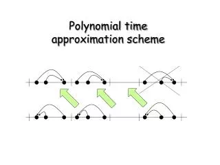
Polynomial time approximation scheme
160 likes | 205 Views
Polynomial time approximation scheme. Polynomial Time Approximation Scheme (PTAS). We have seen the definition of a constant factor approximation algorithm. The following is something even better. An algorithm A is an approximation scheme if for every є > 0,

Polynomial time approximation scheme
E N D
Presentation Transcript
Polynomial Time Approximation Scheme (PTAS) We have seen the definition of a constant factor approximation algorithm. The following is something even better. • An algorithm A is an approximation scheme if for every є > 0, • A runs in polynomial time (which may depend on є) and return a solution: • SOL ≤ (1+є)OPT for a minimization problem • SOL ≥ (1-є)OPT for a maximization problem For example, A may run in time n100/є. There is a time-accuracy tradeoff.
Knapsack Problem A set of items, each has different size and different value. We only have one knapsack. Goal: to pick a subset which can fit into the knapsack and maximize the value of this subset.
Knapsack Problem (The Knapsack Problem) Given a set S = {a1, …, an} of objects, with specified sizes and profits, size(ai) and profit(ai), and a knapsack capacity B, find a subset of objects whose total size is bounded by B and total profit is maximized. Assume size(ai), profit(ai), and B are all integers. We’ll design an approximation scheme for the knapsack problem.
Greedy Methods General greedy method: Sort the objects by some rule, and then put the objects into the knapsack according to this order. Sort by object size in non-decreasing order: Sort by profit in non-increasing order: Sort by profit/object size in non-increasing order: Greedy won’t work.
Dynamic Programming for Knapsack Suppose we have considered object 1 to object i. We want to remember what profits are achievable. For each achievable profit, we want to minimize the size. Let S(i,p) denote a subset of {a1,…,ai} whose total profit is exactly p and total size is minimized. Let A(i,p) denote the size of the set S(i,p) (A(i,p) = ∞ if no such set exists). For example, A(1,p) = size(a1) if p=profit(a1), Otherwise A(1,p) = ∞ (if p ≠ profit(a1)).
Recurrence Formula Remember: A(i,p) denote the minimize size to achieve profit p using objects from 1 to i. How to compute A(i+1,p) if we know A(i,q) for all q? Idea: we either choose object i+1 or not. If we do not choose object i+1: then A(i+1,p) = A(i,p). If we choose object i+1: then A(i+1,p) = size(ai+1) + A(i,p-profit(ai+1)) if p > profit(ai+1). A(i+1,p) is the minimum of these two values.
Running Time The input has 2n numbers, say each is at most P. So the input has total length 2nlog(P). For the dynamic programming algorithm, there are n rows and at most nP columns. Each entry can be computed in constant time (look up two entries). So the total time complexity is O(nP). The running time is not polynomial if P is very large (compared to n).
Approximation Algorithm We know that the knapsack problem is NP-complete. Can we use the dynamic programming technique to design approximation algorithm?
Scaling Down Idea: to scale down the numbers and compute the optimal solution in this modified instance • Suppose P ≥ 1000n. • Then OPT ≥ 1000n. • Now scale down each element by 100 times (profit*:=profit/100). • Compute the optimal solution using this new profit. • Can’t distinguish between element of size, say 2199 and 2100. • Each element contributes at most an error of 100. • So total error is at most 100n. • This is at most 1/10 of the optimal solution. • However, the running time is 100 times faster.
Approximation Scheme Goal: to find a solution which is at least (1- є)OPT for any є > 0. • Approximation Scheme for Knapsack • Given є > 0, let K = єP/n, where P is the largest profit of an object. • For each object ai, define profit*(ai) = profit(ai)/K . • With these as profits of objects, using the dynamic programming algorithm, find the most profitable set, say S’. • Output S’ as the approximate solution.
Quality of Solution Theorem. Let S denote the set returned by the algorithm. Then, profit(S) ≥ (1- є)OPT. • Proof. • Let O denote the optimal set. • For each object a, because of rounding down, • K·profit*(a) can be smaller than profit(a), but by not more than K. • Since there are at most n objects in O, • profit(O) – K·profit*(O) ≤ nK. • Since the algorithm return an optimal solution under the new profits, • profit(S) ≥ K·profit*(S) ≥ K·profit*(O) ≥ profit(O) – nK • = OPT – єP ≥ (1 – є)OPT • because OPT ≥ P.
Running Time For the dynamic programming algorithm, there are n rows and at most n P/K columns. Each entry can be computed in constant time (look up two entries). So the total time complexity is O(n2 P/K ) = O(n3/ є). Therefore, we have an approximation scheme for Knapsack.
Approximation Scheme • Quick Summary • Modify the instance by rounding the numbers. • Use dynamic programming to compute an optimal solution S in the modified instance. • Output S as the approximate solution.
PTAS • Bin Packing • Minimum makespan scheduling • Euclidean TSP • Euclidean minimum Steiner tree But most problems do not admit a PTAS unless P=NP.