Download
1 / 56
560 likes | 731 Views
Routing, Location and Network Design. Marcel Turkensteen ( matu@asb.dk ) CORAL, Aarhus School of Business, Aarhus, Denmark. Introducing myself. Marcel Turkensteen Graduated at the University of Groningen 2002 PhD from the same university in 2007.

E N D
Nizhny Novgorod, presentation 1 Routing, Location and Network Design Marcel Turkensteen (matu@asb.dk) CORAL, Aarhus School of Business, Aarhus, Denmark
Nizhny Novgorod, presentation 1 Introducing myself • Marcel Turkensteen • Graduated at the University of Groningen 2002 • PhD from the same university in 2007. • Now Postdoc at the Aarhus School of Business and Social Sciences.
Nizhny Novgorod, presentation 1 Research interests • Cooperation with Boris Goldengorin on several papers. • Research interests: • Combinatorial Optimization Problems: the use of tolerances in solving them. • Geography and routing / location. • Sustainability and OR. • Sports and OR (starting).
Nizhny Novgorod, presentation 1 Teaching Course that I’ve taught include: • Introduction to Management Science Modeling. • Operations Research methods. • Sustainable Supply Chain Management. • Facility Location and Layout (1 year).
Nizhny Novgorod, presentation 1 Today’s sessions • Presentation 1: Routing, location and network design. • We introduce routing, location and network design problems in logistics. • We introduce the solution approaches to these problems. • Presentation 2: • We discuss how the solution approaches Branch and Bound and Lagrangian relaxation work. • We will introduce and compute tolerance values.
Nizhny Novgorod, presentation 1 The seminar • In the seminar, there are assignments, mainly on the materials from the second presentation.
Nizhny Novgorod, presentation 1 What to learn from both lectures? • Knowing relevant routing and location models in logistics decisions. • Applying simple location and routing heuristics and formulas. • Using Lagrangian relaxation in general: formulating the problem and solving it. • Using Branch and Bound in general: the ingredients. • Learning to compute and analyze upper and lower tolerances.
Nizhny Novgorod, presentation 1 The first presentation - Introduction • If you have a group of dispersed demand points, then what is the costs of supplying products to these demand points? • Ways to model this problem include: • Location problems; • Minimum Spanning Tree Problems. • Location-routing problems; • Vehicle Routing Problems; • Traveling Salesman Problems.
Nizhny Novgorod, presentation 1 • Motivation for this comes from the paper Turkensteen et al. (2011) (Balancing Fit and Logistics Costs…) and a paper with A. Klose (2009). • The question is: what are the logistics costs of serving geographically dispersed demand points? • We modeled the costs using the models discussed in this lecture (in particular the location-routing method).
Nizhny Novgorod, presentation 1 Solution approaches introduced The solution approaches considered here are: • Weiszfeld for single facility location. • The location-routing heuristic by Salhi and Nagy. • The savings heuristic for vehicle routing. • Continuous approximation approaches. • Branch and Bound; • Lagrangian relaxation.
Nizhny Novgorod, presentation 1 Supply chain costs (Ballou, 2004)
Nizhny Novgorod, presentation 1 Expected distribution costs • There are different types of distribution systems: • Multiple echelons versus single echelons; • One-to-many versus many-to-many distribution systems. • The textbook “Logistics system analysis” by Daganzo (2004) summarizes the results on different distribution systems.
Nizhny Novgorod, presentation 1 A logistics costs model • The relevant costs are inventory costs, transportation costs, warehouse costs and handling costs. • How to write it out: transportation costs dependent on travel distances. • Pipeline inventory dependent on travel distances. • Stationary inventory: depends on the dispatch policy. • Warehouse costs: dependent on the number of warehouses. • Handling costs: depending on other operations.
Nizhny Novgorod, presentation 1 Distances and logistics costs • In a one-to-many distribution system, distances influence the logistics costs more or less in a linear way through transportation costs and pipeline inventory costs. • For multi-echelon and many-to-many distribution systems, the number of warehouses and number of echelons influence the logistics costs as well.
Nizhny Novgorod, presentation 1 A set of demand points
Nizhny Novgorod, presentation 1 Problem type 1: Minimum Spanning Tree Problem
Nizhny Novgorod, presentation 1 Minimum Spanning Tree Problems • The Minimum Spanning Tree Problem (MSTP) is the problem of connecting n nodes in a network against minimum costs. • The MSTP can be solved polynomially using e.g. Prim’s algorithm. • An version of the problem discussed in the second lecture is the Degree-Constrained Minimum Spanning Tree Problem, which is NP-hard.
Nizhny Novgorod, presentation 1 Problem type 2: Location problem
Nizhny Novgorod, presentation 1 Where to locate a central facility • Normally, in locating a facility several factors play a role: location of the suppliers, location of customers, regulations, wages, ground prices, etc. • In many location problems, it is assumed that the optimal location is the one that minimizes the sum of the distances to the relevant points. • However, there are many versions of location problems. • Here, we assume that there is a single facility, a continuous plane and the sum of distances needs to be minimized.
Nizhny Novgorod, presentation 1 Minisum Weber Problem • The problem of locating a central facility on a continuous plane is called the minisum Weber problem. • An exact solution approach is Weiszfeld’s algorithm.
Nizhny Novgorod, presentation 1 Weiszfeld algorithm • Weiszfeld’s algorithm is an iterative procedure for solving the minisum Weber problem. • Start with an initial location (x0, y0) • Given location (xk, yk), perform step to end up in location (xk+1, yk+1) • Terminate if satisfying solution is found, or a certain number of iterations has been performed. • In each step, we do: • Drezner (1992): A Note on the Weiszfeld Location Problem.
Nizhny Novgorod, presentation 1 Exercise: the next location is? • Three points with coordinates and weights: 1: (0, 0) with weight 5; 2: (2,1) with weight 3; 3: (5,0) with weight 2. • Start at (1,1). • Take the weighted x-coordinate divided by the distance to the center; divide this by the weights divided by the distance to the center. • Then the new x-coordinate is 5× 0 / √2 + 3× 2 / 1 + 2× 5 / √17 divided by • 5 / √2 + 3/ 1 + 2 / √17 = 1.2. • The y-coordinate becomes ? 0.43
Nizhny Novgorod, presentation 1 More accurate road distances • Distances can be computed with the following formula (lp –norm): • For p = 2, distances are Euclidean. • However, road distances lie in a range between p = 1.5 and p = 3 (see Berens et al, 1985). • This problem can be solved with a generalized version of Weiszfeld algorithm.
Nizhny Novgorod, presentation 1 Generalized Weiszfeld algorithm • For 1 ≤ p < 2, there is a generalized version of the algorithm that converges to the optimal location. • See Brimberg, Chen (1998): A Note on the Convergence of the Single Facility Minisum Location Problem. • For p>2, a transformation exists to transform the problem into the case 1 < p < 2.
Nizhny Novgorod, presentation 1 Location problems: other versions • Location problems with multiple locations are generally more complex than single location problems. • Location problems can be discrete and on networks. • Resulting problems are, among others, p-median problems and simple plant location problems. • An extension is to set up locations such that each demand point is at most M kilometers from a facility (covering problems). • Another extension is to take routing into account when locating facilities: location-routing.
Nizhny Novgorod, presentation 1 Problem type 3: Location routing problems
Nizhny Novgorod, presentation 1 Location-routing problem • In some cases, deliveries to multiple demand points can be combined into single delivery tours (peddling). • It then pays off to jointly decide on location and routes. • It is necessary to decide jointly, because if you don’t take routing into account in the location phase, your location might by (very) suboptimal. • The Location-Routing Problem (LRP) is a very complex problem.
Nizhny Novgorod, presentation 1 Solution methods to the LRP • Exact methods are generally very slow, as the LRP is a very hard problem. • Hierarchical heuristics (location first, then routing), e.g., cluster first, routes later. • The simultaneous location and routing heuristic by Salhi and Nagy (2009).
Nizhny Novgorod, presentation 1 Salhi and Nagy heuristic • Take all demand points and compute the minimum Weber locations of facilities. • Compute the shortest routes given the facilities. • Take the endpoints of the routes. • Compute the minisum Weber locations of facilities with the selected subset of endpoints. • If the locations of the facilities remain the same, terminate, else go to step 2.
Nizhny Novgorod, presentation 1 The heuristic with one facility • The location of the facility in each stage is simply a minisum Weber problem. • The routing from the given facility through the demand point is an example of the next problem: the Vehicle Routing Problem. • With multiple facilities, we should consider the assignments of routes to facilities as well.
Nizhny Novgorod, presentation 1 Remarks on location (Ballou, 2004) • Most current models focus on cost minimization -> how about profit maximization? • Most models are static -> what about a temporal component? • Demand is assumed to be certain -> include demand uncertainty. • Try to include cooperation across the supply chain into the location decision.
Nizhny Novgorod, presentation 1 Problem type 4: Vehicle Routing Problems
Nizhny Novgorod, presentation 1 Vehicle routing • The Vehicle Routing Problem is the problem of constructing a set of tours from a depot to demand points such that the sum of the lengths is minimized. • Usually, there are capacity constraints on the tours, or the number of tours is prescribed. • Solution approaches: … • Savings algorithm; • Meta-heuristics (tabu search); • Exact approaches (column generation).
Nizhny Novgorod, presentation 1 The savings algorithm • The savings algorithm is a simple and very fast algorithm. • It assumes that each route has a certain capacity and each demand point has a certain volume. • First, compute the savings from each connection i to j, s_ij = c_i0 + c_0j – c_ij. • Order the edges on their savings from big to small. • Add edges to routes until no more can be added. • Clarke and Wright (1958).
Nizhny Novgorod, presentation 1 Problem type 5: Traveling salesman Problems
Nizhny Novgorod, presentation 1 Traveling Salesman Problem • The Traveling Salesman Problem (TSP) is the problem of finding a minimum length tour through n locations, such that each locations is visited exactly once. • Asymmetric (ATSP): the distance from i to j is not necessarily equal to the distance from j to i. • The ATSP is presented extensively in lecture 2 in combination with Branch and Bound.
Nizhny Novgorod, presentation 1 TSP solution approaches • For the Symmetric version of the problem: • The exact Concorde approach (Branch-and-Cut); • Meta-heuristics such as the modified Lin-Kernighan Variable Neighborhood Search heuristic from Helsgaun (2000). • Asymmetric: • Branch and Bound type methods, see second lecture. • Cut and Solve.
Nizhny Novgorod, presentation 1 Solution approach: Continuous approximation • Estimate distribution costs given a uniform distribution of demand points in a certain area. • Estimation of route lengths within TSP, VRP, and LRP. • We discuss main results. • One warehouse vs multiple warehouses.
Nizhny Novgorod, presentation 1 Continuous Approximation • Eilon (1971) found the following TSP tour length estimate: • The assumption is that the demand locations are randomly (uniformly) distributed across a certain area. • Here, k is a constant for the type of distances, e.g., 0.57 for Euclidean and 0.72 for rectilinear.
Nizhny Novgorod, presentation 1 Continuous Approximation • Extended to systems with VRP tours with a most C stops in Daganzo (2004), Langevin (1996): • Here E(δ^(-1/2) is the density of the area, and E(r) the average distance to a central point in the area. • If demand points are uniformly distributed and C sufficiently large, the formula is:
Nizhny Novgorod, presentation 1 Estimate tour lengths • Consider the data set with N = 25, the maximum difference between x-coordinates is 40 and between y-coordinates is 25. • Assume Euclidean distances. • Compute the: • Estimated tour length; • The estimated VRP route length for C=2. • The estimated VRP route length for C=10.
Nizhny Novgorod, presentation 1 Validity of continuous approximation results • Continuous approximation results are valid in areas with different shapes (Daganzo, 1984), with time windows on routes (Figliozza, 2008). • The results are extended to transshipment warehouses in Daganzo (1986) and Campbell (1993). • A more or less uniform distribution is assumed. • In some studies, the results serve as a starting point for further optimization; see e.g. Robuste et al. (1990).
Nizhny Novgorod, presentation 1 Our studies • We tried to devise simple measures of demand dispersion in order to estimate route lengths. • In one-to-many distribution systems, route lengths are closely related to the logistics costs. • We used continuous approximation results to come up with distance measures. • For C=1, it is a regular location problem, whereas for C > 2, we have an LRP or a VRP. • We find that travel distance estimates can be very accurate. • In one paper, we include such a measure within a market research method.
Nizhny Novgorod, presentation 1 Conclusion and summary • The first lecture discusses a wide range of topics within logistics network. • We started with discussing logistics costs and relating them to OR problems. • Then we discussed problem and methods within location, routing and network design. • Methods discussed in more detail are Weiszfeld’s algorithm, the savings algorithm and a location-routing method.
Nizhny Novgorod, presentation 1 References • Ballou, R. (2001) Unresolved Issues in Supply Chain Network Design. Information Systems Frontiers 3(4), 417–426. • Bektas, T. and Laporte, G. (2001) The Pollution-Routing Problem, Transportation Science. • Clarke, G. and Wright, J. (1964) Scheduling of Vehicles from a Central Depot to a Number of Delivery Points. Operations Research 12, 568–581. • Daganzo, C. (1984) The Distance Traveled to Visit N Points with a Maximum of C Stops per Vehicle: An Analytic Model and an Application. Transportation Science 18, 331–350.