Download
1 / 25
280 likes | 503 Views
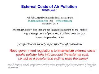
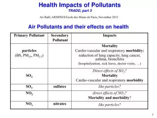
Atmospheric models for damage costs TRADD, part 2. Ari Rabl, ARMINES/ Ecole des Mines de Paris , November 2013 There are many different models for atmospheric dispersion and chemistry, with different objectives : e.g. microscale models (street canyons),

E N D
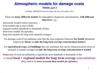
Atmospheric models for damage costsTRADD, part 2 Ari Rabl, ARMINES/Ecole des Mines de Paris, November 2013 There are many different models for atmospheric dispersion and chemistry, with different objectives: e.g. microscale models (street canyons), local models (up to tens of km), regional models (hundreds to thousands of km), short term models for episodes, long term models for long term (annual) averages. For damage costs of air pollution, note that the dose-response functions for health (dominant impact) are linear only the long term average concentration matters For agricultural crops and buildings they are nonlinear, but can be characterized in terms of seasonal or annual averages only the long term average concentration is needed Dispersion of most air pollutants is significant up to hundreds or thousands of km need local + regional models for long term average concentrations (they tend to be more accurate than models for episodes)
Depends on meteorological conditions: wind speed and atmospheric stability class (adiabatic lapse rate, see diagrams at left) Dispersion of Air Pollutants
for atmospheric dispersion (in local range < ~50 km) Gaussian plume model
Underlying hypothesis: fluid with random fluctuations around a dominant direction of motion (x-direction) Gaussian plume model, concentration c at point (x,y,z) c=concentration, kg/m3 Q=emission rate, kg/s v= wind speed, m/s, in x-direction y=horizontal plume width z=vertical plume width he=effective emission height Source at x=0,y=0 Plume width parameters y and zincrease with x
There are several models for estimating y and zas a function of downwind distance x, for example the Brookhaven model Gaussian plume width parameters where To use model one needs data for wind speed and direction, and for atmospheric stability (Pasquill class); the latter depends on solar radiation and on wind speed.
Gaussian plume with reflection terms When plume hits ground or top of mixing layer, it is reflected
Effect of stack parameters Plume rise: fairly complex, depends on velocity and temperature of flue gas, as well as on ambient atmospheric conditions
Influence of Emission Source Parameters and Meteorological Data on Damage Estimates. The Source is Located in a Suburb of Paris. Effect of stack parameters, examples
Mechanisms for removal of pollutants from atmosphere: 1) Dry deposition (uptake at the earth's surface by soil, water or vegetation) 2) Wet deposition (absorption into droplets followed by droplet removal by precipitation) 3) Transformation (e.g. decay of radionuclides, or chemical transformation SO2NH4)2SO4). They can be characterized in terms of deposition velocities, (also known as depletion or removal velocities) vdep = rate at which pollutant is deposited on ground, m/s (obvious intuitive interpretation for deposition) vdep depends on pollutant determines range of analysis: the smaller vdep the farther the pollutant travels) Typical values 0.2 to 2 cm/s for PM, SO2 and NOx Gaussian plume model can be adapted to include removal of pollutants Removal of pollutants from atmosphere
Far from sourcegaussian plume with reflections implies vertically uniform concentrations Therefore consider line source for regional dispersion (point source and line source produce same concentration at large r) Assume wind speed is always = v, uniform in all directions f Regional Dispersion, a simple model the pollutant spreads over an area that is proportional to r
Consider mass balance as pollution moves from r to r+r, if uniformity in all directions • mass flow v c(r) H r across shaded surface at r • = mass flow v c(r+r) H (r+r) across shaded surface at r+r • + mass vdep c(r +r/2) r (r+r/2) deposited on ground between r and r+r • Taylor expand c(r+r) = c(r) + c’(r) r and neglect higher order terms • Differential equation c’(r) = - ( + 1/r) c(r) with = vdep/(v H) Simple model for regional dispersion, cont’d Solution c(r) = c0exp(- r)/rwith constant c0 to be determined
Determination of c0 by considering integral of flux v c(r) over cylinder of height H and radius r in limit of r 0 This integral must equal to emission rate Q [in kg/s]. Hence Simple model for regional dispersion, cont’d Therefore final result with This model can readily be generalized (i) To case where wind speeds in each direction are variable with a distribution f(v(), ) with normalization (ii) To case where trajectories of puffs meander instead of being straight lines: then exp(- r) is replaced by exp(- t(r)) where t(r) = transit time to r; all else remains the same.
Total impact I = integral of sER c(r) • with = receptor density and sER = slope of exposure-response function • Simple case: and sER independent of r and with Impact vs cutoff rmax with If cutoff rmax for integral Range 1/ = v H/vdep = 800 km for mixing layer height H = 800 m wind speed v = 10 m/s depletion velocity vdep = 0.01 m/s
Primary pollutants (emitted) secondary pollutants aerosol formation from NO, SO2 and NH3 emissions. Chemical Reactions Note: NH3 background, mostly from agriculture
Product of a few factors (dose-response function, receptor density, unit cost, depletion velocity of pollutant, …), • Exact for uniform distribution of sources or of receptors • UWM (“Uniform World Model”) for inhalation • verified by comparison with about 100 site-specific calculations by EcoSense software (EU, Eastern Europe, China, Brazil, Thailand, …); • recommended for typical values for emissions from tall stacks, more than about 50 m (for specific sites the agreement is usually within a factor of two to three; but for ground level emissions the damage of primary pollutants is much larger: apply correction factors). • UWM for ingestion is even closer to exact calculation, because food is transported over large distances average over all the areas where the food is produced effective distributions even more uniform. • Most policy applications needtypical values • (people tend to use site specific results as if they were typical • precisely wrong rather than approximately right) UWM: a simple model for damage costs
Total impact I = integral of sER c(x) over all receptor sites x = (x,y) • with • c(x) = c(x,Q) = concentration at surface due to emission Q Q • (x) = density of receptors (e.g. population) • sER= slope of exposure-response function • Total depletion flux (due to deposition and/or transformation) • F(x) = Fdry(x) + Fwet(x) + Ftrans(x) • Define depletion velocityvdep(x) = F(x)/c(x) [units of m/s] • Replace c(x) in integral by F(x)/k(x) • If world were uniform with • uniform density of receptors and uniform depletion velocity vdep • then • By conservation of mass • “Uniform World Model” (UWM) for damage UWM: derivation
dependence on site and on height of source for a primary pollutant: impact I from SO2 emissions with linear exposure-response function, for five sites in France, in units of Iuni for uniform world model (the nearest big city, 25 to 50 km away, is indicated in parentheses). The scale on the right indicates YOLL/yr (mortality) from a plant with emission 1000 ton/yr. Plume rise for typical incinerator conditions is accounted for. UWM and Site Dependence, example
Factor of two Comparison with detailed model (EcoSense = official model of ExternE) Validation of UWM, for primary pollutants
Same approach: add a subscript 2 to indicate that concentration, dose-response function and damage refer to the secondary pollutant UWM for secondary pollutants
Let us relate Q2 to the emission Q1 of the primary pollutant: define a creation flux F1-2(x) as mass of secondary pollutant created per s and per m2 of horizontal surface F1-2(x) = v1-2(x) c1(x) where v1-2(x) is a factor defined as local ratio of F1-2(x) and c1(x). UWM for secondary pollutants, cont’d Therefore UWM for secondary pollutants with
Strongvariation for primary pollutants but little variation for secondary pollutants, because created far from source (hence less sensitive to local detail) Dependence site and on stack height
Correction factors for UWM for dependence on site and on stack height No variation with site for CO2 (long time constants, globally dispersing) Example: the cost/kg of PM2.5 emitted by a car in Paris is about 15 times Duni.
Population density and depletion velocities, in cm/s, selected data for several regions. From Rabl, Spadaro and Holland [2013] Parameters for UWM