Download
1 / 30
300 likes | 493 Views
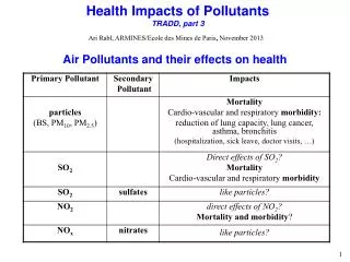
Health Impacts of Pollutants TRADD, part 3. Ari Rabl, ARMINES/Ecole des Mines de Paris , November 2013. Air Pollutants and their effects on health. Air Pollutants and their effects on health , cont ’ d.

E N D
Health Impacts of PollutantsTRADD, part 3 Ari Rabl, ARMINES/Ecole des Mines de Paris, November 2013 Air Pollutants and their effects on health
Healthy individuals have sufficient reserve capacity not to notice effects of pollution, but the effects become observable at times of low reserve (during extreme physical stress, severe illness, or last period of life) Cardio-pulmonary effects of air pollution Pollution reduces reserve capacity Mortality impact is not the loss of a few months of misery at the end but the shrinking of the entire quality of life curve (“accelerated aging”) In large population there are always some individuals with very low reserve capacity impacts observable
Air pollution mortality is closely linked to morbidity and quality of life. An individual who dies prematurely due to air pollution loses not just a few months of poor health at the end of life, but suffers an impairment of general health during the entire period of exposure and this impairment can considerably affect the quality of life, especially for people who are old or already in poor health. For example, a young person with 4 l lung capacity can survive very well with a 0.5 l decrease but if the capacity is already as low as 1.5 l such a decrease causes serious problems. Even though air pollution can affect everybody’s health, the effects are observable onlyamong the most vulnerable, typically the very young, the old and the sick. And of course, even the young will be old someday. The identified ERFs, and the corresponding monetary values, are only proxies for the real impact of air pollution; it is not entirely clear to what extent they cover all the important impacts or involve double counting. This type of uncertainty involves subjective judgment rather than formal analysis. Mortality,morbidity, gaps and double counting
Epidemiology: comparing populations with different exposures. 2) Laboratory experiments with humans: exposure in test chambers with controlled concentration of air pollutants (but this approach is very limited because of ethical constraints). 3) Toxicology: a) Expose animals (usually rats or mice) to a pollutant; sample sizes are usually very small compared to epidemiological studies, and the animals are selected to be as homogenous as possible (unlike real populations). Extrapolation to humans??? b) Expose tissue cultures to pollutants. Extrapolation to real organism??? Approaches to measure health impacts
Epidemiology: can measure impacts on real human populations, by observing correlations (“associations”) between exposure and impact. But in most cases the uncertainties are very large. Is the impact due to the pollutant or due to other variables that have not been taken into account (the problem of “confounders”, especially smoking)? Toxicology: can identify mechanisms of action of the pollutants. For many substances toxicology is the only way to identify carcinogenic effects. Toxicology can also suggest new questions to be investigated by epidemiology. The two approaches are complementary. Approaches to measure health impacts, cont’d
1) Time series (only for air pollution): Observe correlations, in a large city, between concentration and occurrence of health impacts during the following days (in practice at most during the following five days). Advantage: inexpensive; most confounders (especially smoking) are eliminated. Disadvantage: only acute effects can be observed. 2) Cohort studies: Compare different populations, using detailed information on the individuals to minimize effect of confounders. Advantage: can observe chronic effects. Disadvantage: expensive; often requires observations over many years; confounders are difficult to eliminate. There are other types, and several variants, e.g. observation of population during a large and permanent change of exposure (e.g. Dublin and Hong before and after new regulation on use of certain fuels). Types of epidemiological studies
3) Intervention studies: If due to some intervention the exposure to a pollutant was reduced during an extended period (at least a year), one can compare the health impacts before and after. Unfortunately this kind of situation occurs only rarely, and there are only three unambiguous cases for air pollution: Closure of large steel mill in Utah Valley for 13 months 1986/87. Regulation banning the use of high sulfur fuel in Hong Kong after July 1990 Regulation banning the use of coal in Dublin after July 1990 In all of these cases significant reductions in mortality and morbidity were observed. Types of epidemiological studies
(also known as dose-response functions or concentration response functions) Crucial for calculating impacts of a pollutant Form of exposure-response functions at low doses Possible functional forms at low doses Linearity without threshold is the most plausible assumption for NO2, PM, O3, SO2, and carcinogens
The problem: in most regions the concentrations are so low that their impacts are difficult or impossible to measure. Suppose P is the lowest concentration where an impact could be measured with reasonable accuracy. How should one extrapolate to lower exposures? • All of these functional forms can occur, for example • linear: radioactivity, particulates health • threshold: ozone crops • fertilizer: SO2 for crops • but very few above linear in low dose limit. • Linearity without threshold seems to be the most plausible for health impacts of air pollutants, for IQ decrement due to Pb, and for substances that initiate cancers (also for radioactivity). Functional form of exposure-response functions at low exposures, cont’d
Is it Causal?Hill's criteria for causality of statistical correlations ("associations") found in epidemiological studies
but uncertainties about some specifics, in particular which pollutant causes which effects. The dominant opinion in the USA has been that PM and O3 are the main culprits, but recent results suggest that direct effects of SO2 and NO2 may also be important. Major uncertainty: toxicity of components of PM Quite variable, typically soot and other direct combustion particles 10 to 30% soil particles 10 to 50% (wind blown or stirred up by human activities) sulfates 10 to 50% nitrates 10 to 30% Some nitrates and sulfates are of natural origin What is relative toxicity of soil particles, nitrates and sulfates? Role of other characteristics (acidity, solubility, surface area, number of particles, detailed composition)? Synergistic effects? Slow convergence towards a consensus : "air pollution is harmful to your health"
relative risk RR = m/m0 where m0 = mortality at a reference concentration c0 , m = mortality at concentration c There are several different definitions of mortality rates: (i) Time series determine the relative risk RR of acute exposure for the daily mortality m [deaths/day] of the total population, or in some case for a subgroup e.g. people over 65 Typical value RR - 1 = 0.06% per g/m3 of PM10. (ii) Cohort studies determine the relative risk RR of chronic exposure for the age-specific mortality m(x) [probability/yr] which is defined as the probability for an average person of age x to die during the coming year; if the rate at a reference concentration c0 is m0, at concentration c it is m = RR m0. Typical value RR – 1 = 0.6% per g/m3 of PM2.5, (or RR - 1 = 0.36% per g/m3 of PM10, for typical ratio PM2.5/PM10 = 0.6). The values of R are very different because they measure different effects: “acute mortality” for time series, total “chronic mortality” for cohort studies. Calculation of life expectancy
Survival function S(x,x’) = fraction of a cohort of age x that survives at least to age x’. Since the fraction that dies between x’ and x’ + x’ is S(x,x’) = S(x,x’) (x) x, differential equation dS(x,x’) = - S(x,x’) (x’) dx’ with boundary condition S(x,x) = 1. Solution Calculation of life expectancy, cont’d The probability distribution for a member of the age x cohort to survive to and die at age x’ is p(x,x’) = S(x,x’) (x’) , normalized to unity over the interval from x to . The expected age of death is the integral of x’ p(x,x’) from x to . The difference between the expected age of death and the starting age x is the remaining life expectancy L(x) of this cohort For practical calculations integrate by parts and approximate by annual values from life tables.
For example, a fraction 0.6 of the population survives to 81 yr and a fraction 0.5 to 84 yr. A fraction 0.6 - 0.5 = 0.1 dies between these ages, at about x’ = 82.5 on average; this corresponds to a horizontal slice under the survival curve between S(0,x’) = 0.5 and 0.6. Calculation of life expectancy, cont’d Life expectancy at birth
Calculation of life expectancy (LE), cont’d Survival probability S(0,x) for surviving to age x. Solid line = S0(0,x) for (x) with life expectancy LE = 75 yr; dotted line = SR(0,x) for (x) = RR (x) with rel.risk RR=1.17 LE = 73.4 yr (these are older data: LE has been increasing by 2 to 3 yr per decade, now about 80 yr in France)
If (x) changes due to air pollution, S(x,x’) and L(x) change accordingly. The resulting LE loss DLE(x) for a cohort of age x is the difference between L(x) calculated without and with this increase Calculation of life expectancy, cont’d where S0(x,x’) is the survival curve for the baseline mortality 0(x). The impact on the entire population is obtained by summing DLE(x) over all affected cohorts, weighted by the age distribution (x) In practice for adult mortality the lower limit is replaced by 30 because the cohort studies have considered only people over 30 and mortality is low below 30.
Calculation of life expectancy, cont’d The age distribution (x) for EU15 for 1997, USA for 1996, and a stationary population with total mortality of EU15.
Loss of Life Expectancy (LE) due to Air Pollution In EU and USA typical concentrations of PM2.5 around 20 - 30 g/m3LE loss 8 months Reasonable policy goal during coming decades: reduction by about 50% LE gain about 4 months To put this in perspective with other public health risks: Smokers lose about 5 to 8 years on average Rule of thumb: each cigarette reduces LE by about the duration of the smoke Air pollution (in EU and USA) equivalent to about 4 cigarettes/day
Gain of life expectancy LE (population average, per person)for reduction of PM10 concentration by 15 g/m3calculated by Rabl, J Air&Waste Management Assoc. Vol.53(1), 41-50 (2003), on the basis of the indicated references. Results for change in life expectancy LE • ERF slope for total mortality, in YOLL per year of exposure per mg/m3 of PM2.5 • sER= 4.56E-4 YOLL/(yrµgPM2.5/m3)
ERF slope for total mortality, in YOLL per year of exposure per mg/m3 of PM2.5 • sER= 4.56E-4 YOLL/(yrµgPM2.5/m3) Example: PM10 concentrations in Chinese cities averaged about 300 mgPM10/m3 during the nineteen seventies and by 2005 they had decreased to 100 mgPM10/m3. What is the current loss of LE per year of exposure? Solution: Not having data for PM2.5, we assume a typical conversion factor of about 0.6 for the ratio of PM2.5 and PM10 concentrations. Thus the loss is 0.6 *100 mgPM10/m3 * 4.56E-4 YOLL/(yrµgPM2.5/m3) = 0.027 YOLL/yr = 0.3 months per year of exposure. For a constant exposure at this level during an entire 73 yr lifespan (the LE in China around 2010) the loss would be 73 yr * 0.027 YOLL/yr= 2 years of life lost. Change in life expectancy LE, an example
Impacts (“end points”) for which there are ERFs (i) Chronic impacts CB = chronic bronchitis (another impact is reduced lung function, but there is no monetary valuation). (ii) Acute impacts HA = hospital admission LRS = lower respiratory symptoms mRAD = minor restricted activity day RAD = restricted activity day URS = upper respiratory symptoms WDL = work days lost Some of these impacts have been identified for asthmatics (about 4 to 6% of total population in industrialized countries, incidence has been increasing in recent years) Morbidity
ERF slopes and monetary values YOLL = years of life lost
Example: in Paris in 2010 the annual mean PM2.5 concentration has been about 20 mgPM2.5/m3 in most areas, and the affected population is about 2.5 million. How large is the value of the health gain if the concentration is reduced to 15 mgPM2.5/m3? Example: value of air quality improvement
Example: According to COPERT4 software, PM2.5 emissions for EURO5 (in force since Jan. 2011) cars in city driving are about 0.013 g/km (essentially the same for diesel and for gasoline). How large is the damage cost per km? Solution: Use the UWM with r = 100 persons/km2 and vdep = 0.005 m/s, and assume that the damage for ground level emissions in Paris is 15 times larger. Careful about units: Iuni = impact rate for Q = emission rate, hence assume 1 km/yr: Q = 0.013 g/yr = Example: cost of PM emission by car in Paris
The EURO standards for emission limits of passenger cars, in g/km. EURO standards * Applies only to vehicles with direct injection engines THC = total hydrocarbons, NMHC = nonmethane hydrocarbons
1 ppb O3 = 1.997 g/m3 of O3 1 ppb NO2 = 1.913 g/m3 of NO2 1 ppm CO = 1.165 mg/m3 of CO BS = black smoke c = concentration CB = chronic bronchitis COPD = chronic obstructive pulmonary disease DRF = dose-response function, also known as concentration-response (CR) function and exposure-response function (ERF) ERF = exposure-response function EPA = Environmental Protection Agency of USA fpop = fraction of the population affected by the end point in question. HA = hospital admission Iref.= baseline or reference level of incidence of the end point in question. LLE = loss of life expectancy LRS = lower respiratory symptoms mRAD = minor restricted activity day NOx = unspecified mixture of NO and NO2 PMd = particulate matter, with subscript d indicating that only particles with aerodynamic diameter below d, in m, are included RR = relative risk RAD = restricted activity day sER= slope of ERF URS = upper respiratory symptoms VOC = volatile organic compounds WDL = work day lost YOLL = years of life lost = coefficient of Gompertz function for mortality = coefficient of Gompertz function for mortality = ln(R)/c R/c c = change in concentration. RR = change in relative risk Glossary and conversion factors
Abbey DE, N Nishino, WF McDonnell, RJ Burchette, SF Knutsen, WL Beeson and JX Yang 1999. "Long-term inhalable particles and other air pollutants related to mortality in nonsmokers". Am. J. Respir. Crit. Care Med., vol. 159, 373-382. Bobak M and DA Leon 1999. "The effect of air pollution on infant mortality appears specific for respiratory causes in the postneonatal period". Epidemiology 10(6), 666-670. Clancy L, Pat Goodman, Hamish Sinclair, Douglas W Dockery. 2002. “Effect of air-pollution control on death rates in Dublin, Ireland: an intervention study”. Lancet, vol.360, October 19. Dockery DW, CA Pope III, XipingXu, JD Spengler, JH Ware, ME Fay, BG Ferris & FE Speizer 1993. "An association between air pollution and mortality in six US cities". New England J of Medicine, vol.329, p.1753-1759 (Dec. 1993). Hedley AJ, Chit-Ming Wong, ThuanQuocThach, Stefan Ma, Tai-Hing Lam, Hugh Ross Anderson. 2002. “Cardiorespiratory and all-cause mortality after restrictions on sulphur content of fuel in Hong Kong: an intervention study”, Lancet, vol.360, November 23. Hoek G, Bert Brunekreef, Sandra Goldbohm, Paul Fischer and Piet A van den Brandt. 2002. “Association between mortality and indicators of traffic-related air pollution in the Netherlands: a cohort study”. The Lancet, Vol.360 (Issue 9341, 19 October), 1203-1209. Katsouyanni K, Touloumi G, Spix C, Schwartz J, Balducci F, Medina S, Rossi G, Wojtyniak B, Sunyer J, Bacharova L, Schouten JP, Ponka A, Anderson HR. 1997. “Short-term effects of ambient sulphur dioxide and particulate matter on mortality in 12 European cities: Results from time series data from the APHEA project.” British Med. J 314:1658–1663. Pope CA, RT Burnett, MJ Thun, EE Calle, D Krewski, K Ito, & GD Thurston 2002. "Lung cancer, cardiopulmonary mortality, and long term exposure to fine particulate air pollution ". J. Amer. Med. Assoc., vol.287(9), 1132-1141. Rabl A 2003. “Interpretation of Air Pollution Mortality: Number of Deaths or Years of Life Lost?”. J Air and Waste Management, Vol.53(1), 41-50 (2003). Samet JM, Dominici F, Zeger SL, Schwartz J, Dockery DW. 2000a. “The National Morbidity, Mortality and Air Pollution Study, Part I: Methods and Methodologic Issues.” Research Report 94, Part I. Health Effects Institute, Cambridge MA. Available at http://www.healtheffects.org/ Samet JM, F Dominici, FC Curriero, I Coursac & SL Zeger. 2000b. “Fine Particulate Air Pollution and Mortality in 20 U.S. Cities, 1987–1994”. N Engl J Medicine, vol.343(24), 1742-1749. Woodruff TJ, Grillo J, Schoendorf KC 1997. “The relationship between selected causes of postneonatal infant mortality and particulate air pollution in the United States”. Environ Health Perspect, vol.105(6), 608-612. References