Introduction to Optical Fibre Principles
690 likes | 1.14k Views
Introduction to Optical Fibre Principles. Wavelength and Spectra. Wavelength: Light can be characterised in terms of its wavelength Analogous to the frequency of a radio signal The wavelength of light is expressed in microns or nanometers

Introduction to Optical Fibre Principles
E N D
Presentation Transcript
Wavelength and Spectra • Wavelength: • Light can be characterised in terms of its wavelength • Analogous to the frequency of a radio signal • The wavelength of light is expressed in microns or nanometers • The visible light spectrum ranges from ultraviolet to infra-red • Optical fibre systems operate in three IR windows around 800 nm, 1310 nm and 1550 nm 400 200 600 800 1000 1200 1400 1600 1800 Visible light Fibre operating windows Spectrum of light (wavelength in nanometers)
Advantages and Disadvantages Advantages • Low attenuation, large bandwidth allowing long distance at high bit rates • Small physical size, low material cost • Cables can be made non-conducting, providing electrical isolation • Negligible crosstalk between fibres and high security, tapping is very difficult • Upgrade potential to higher bit rates is excellent Disadvantages • Jointing fibre can be more difficult and expensive • Bare fibre is not as mechanically robust as copper wire • Fibres are not directly suited to multi-access use, alters nature of networks • Higher minimum bend radius by comparison with copper
Applications for Fibre in Buildings Horizontal Cabling Building Backbone • Most fibre is used in campus and building backbones • Horizontal cabling is mainly copper at present but may become fibre Campus Backbone
How does Light Travel in a Fibre? Optical Fibre Transmitter Electrical output signal Receiver Light ray trapped in the core of the fibre Electrical input signal
Fibre Types • Three generic fibre types dominate the building cable market • Multimode is most popular but singlemode is now being installed more frequently • Multimode is more tolerant of source and connector types • Singlemode offers the largest information capacity Multimode fibre Multimode fibre Singlemode fibre 125 microns cladding diameter 62.5 micron core diameter 50 micron core diameter 8 micron core diameter
Decibels and Attenuation Basic decibel power equation relates two absolute powers P1 and P2: Power ratio in dB = 10 Log [P1/P2] 10 In a fibre or other component with an input power Pin and an output power Pout the loss is given by: Loss in dB = 10 Log [Pout/Pin] 10 By convention the attenuation in a fibre or other optical component is specified as a positive figure, so that the above formula becomes: Attenuation in dB = -10 Log [Pout/Pin] 10
Absolute power in Decibels • It is very useful to be able to specify in dB an absolute power in watts or mW. • To do this the power P2 in the dB formula is fixed at some agreed reference value, so the dB value always relates to this reference power level. • Allows for the easy calculation of power at any point in a system Where the reference power is 1 mW the power in an optical signal with a power level P is given in dBm as: Power in dBm = 10 Log [P/1mW] 10 For example 2 mW is +3 dBm, 100 µW is -10 dBm and so on. Negative dBm simply means less than 1 mw of power. 1 mW is 0 dBm
Watts to dBm Conversion Table Power (watts) Power (dBm) 1 W +30 dBm 100 mW +20 dBm 10 mW +10 dBm 5 mW +7 dBm 2 mW +3 dBm 1 mW 0 dBm 500 mW -3 dBm 200 mW - 7 dBm 100 mW -10 dBm 50 mW -13 dBm 10 mW -20 dBm 5 mW -23 dBm 1 mW -30 dBm 500 nW -33 dBm 100 nW -40 dBm
Attenuation in Fibre: Transmission Windows • Three low loss transmission windows exist circa 850, 1320, 1550 nm • Earliest systems worked at 850 nm, latest systems at 1550. 1st window circa 850 nm 2nd window circa 1320 nm 3rd window circa 1550 nm Loss dB/Km 10 1 Wavelength in nanometers 0.1 600 700 800 900 1000 1100 1200 1300 1400 1500 1600
Bending Loss in Fibres • At a bend the propagation conditions alter and light rays which would propagate in a straight fibre are lost in the cladding. • Macrobending, for example due to tight bends • Microbending, due to microscopic fibre deformation, commonly caused by poor cable design Microbending is commonly caused by poor cable design Macrobending is commonly caused by poor installation or handling
Types of Optical Fibre • Three distinct types of optical fibre have developed • The three fibre types are: • Step index fibre • Graded index fibre • Singlemode fibre (also called monomode fibre) Multimode fibres
Dispersion in an Optical Fibre • Fibre type influences so-called "Dispersion" • The higher the dispersion the lower the fibre bandwidth • Lower fibre bandwidths mean less information capacity Modal Dispersion: Reduced by using graded index fibre Eliminated by using singlemode fibre Material Dispersion: Reduced by using Laser rather than LED sources Reduced by operating close to 1320 nm
Multimode Fibre Bandwidth (I) • Combination of modal and material dispersion limits fibre bandwidth • Dispersion is rarely specified, bandwidth is more useful • Typically stated as MHz.km • For example ISO 11801 specifies 500 MHz.km for 50/125 µm fiber in the 1300 nm window • Bandwidths range from about 200 MHz.km to 2000 MHz.km. • 50/125 µm fibre will have higher bandwidth than 62.5/125 µm fibre
Multimode Fibre Bandwidth (II) • To find the bandwidth of a fibre span, divide the bandwidth in MHz.km by the fibre span in km. • The longer the fibre span, the lower the overall bandwidth. Example: Assume a fibre bandwidth of 600 MHz.km Overall bandwidth = 375 MHz Fibre span = 1.5 km Overall bandwidth = 666 MHz 0.9 km Overall bandwidth = 2400 MHz 250 m
Multimode Fibre Bandwidth and Bit Rate in LANs • Relationship between available bandwidth and maximum bit rate is complex • For LANs and building cabling systems rule is (from standards): Fibre bandwidth in MHz.km Maximum bit rate in MB/s = 2 x Fibre span in km • Rule is very conservative, assumes zero dispersion penalty is required • For example for a 500 MHz.km over 2000 m the maximum bit rate is 125 MB/s • In practice use a fibre that exceed the standards for a given LAN to ensure adequate bandwidth
Summary • Optical fibre systems utilise infared light in the range 700 nm to 1600 nm • Fibre has a number of significant advantages • Building fibre systems operate around 1320 nm • Multimode fibres suffer from modal and material dispersion • Material dispersion is minimised by operating near 1320 nm • Singlemode fibre eliminates material dispersion
Planning Fibre Systems: Standards & Power Budgeting in Local Area Networks
Relevant standards • Power budget definition • Power margins • Sample exercises
EN 50173: Functional Elements • EN 50173 Information technology - Generic cabling systems • A number of functional elements are defined: • Campus Distributor (CD) • Campus Backbone Cable • Building Distributor (BD) • Building Backbone Cable • Floor Distributor (FD) • Horizontal Cable • Transition Point (optional) TP • Telecommunications Outlet (TO) Krone
EIA/TIA 568-B and Fibre • EIA/TIA 568-B 2001 Commercial Building Telecommunications Wiring Standard • This is an American Standard • International and European standards used this as their basis • Recognises 62.5/125 micron fibre for horizontal cabling • Recognises 62.5/125 micron fibre and singlemode fibre for backbones • Section 12 of the standard covers fibre specs • No longer specifies a particular connector type but sets minimum standards the connector must meet • Maximum mated pair connector attenuation is 0.75 dB • Maximum splice loss for fusion or mechanical is 0.3 dB • Different colour coding for multimode and singlemode connectors
ISO 11801:2002 • Information technology -- Generic cabling for customer premises • ISO/IEC 11801 specifies generic cabling for use within premises, which may comprise single or multiple buildings on a campus. It covers balanced cabling and optical fibre cabling. • ISO/IEC 11801 is optimised for premises in which the maximum distance over which telecommunications services can be distributed is 2000 m. The principles of this International Standard may be applied to larger installations. • Cabling defined by this standard supports a wide range of services, including voice, data, text, image and video. • This International Standard specifies directly or via reference the: • structure and minimum configuration for generic cabling, • interfaces at the telecommunications outlet (TO), • performance requirements for individual cabling links and channels, • implementation requirements and options, • performance requirements for cabling components required for the maximum distances specified in this standard, • conformance requirements and verification procedures. • Safety (electrical safety and protection, fire, etc.) and Electromagnetic Compatibility (EMC) requirements are outside the scope of this International Standard, and are covered by other standards and by regulations. However, information given by this standard may be of assistance. • ISO/IEC 11801 has taken into account requirements specified in application standards listed in Annex F. It refers to available International Standards for components and test methods where appropriate
According to ISO – 11801 International Standards Organization OM1 fiber – 200/500 MHz.km OFL BW (in practice OM1 fibers are 62.5 μm fibers) OM2 fiber – 500/500 MHz.km OFL BW (in practice OM2 fibers are 50 μm fibers) OM3 fiber – Laser-optimized 50 mm fibers with 2000 MHz.km EMB at 850 μm Fibre Types in LANs
According to ISO 11801 Maximum channel length varies between 300m to 2000m depending on the application Specific applications are bandwidth limited at the channel lengths shown in the standard document For example ATM running over a 50μm fiber ATM 155 Mbits/s @ 850nm 1000m ATM 622 Mbits/s @ 850nm 300m ATM 155 Mbits/s @ 1300nm 2000m ATM 622 Mbits/s @ 1300nm 330m Maximum Distances
ISO 11801 Optical fibre cable attenuation ISO 11801:2002 Note:Attenuation is in dB/km
Class OF-300 Supports applications to a minimum of 300m Class OF-500 Supports applications to a minimum of 500m Class OF-2000 Supports applications to a minimum of 2000m ISO 11801 Optical fibre Channel Classes
ISO 11801 Optical fibre Channel Attenuation The channel attenuation shall not exceed the values shown in the table above. The values are based on a total allocation of 1.5dB for connecting hardware. ISO 11801:2002
11801 Standards for Fibre Joints in Buildings • For connectors maximum mated pair connector attenuation is 0.75 dB • Different colour coding for multimode and singlemode connectors • Maximum splice loss for fusion or mechanical is 0.3 dB Mated pair of ST type Optical Connectors
Building Cabling Connectors and Standards • Presently the ST-compatible connector and SC-compatible connector are the most commonly used connectors for termination. • ISO 11801 nolonger specifies a specific connector type but points to a minimum set of specifications that an optical connector must meet. • The primary advantages of the SC connector are: • It is a duplex connector, which allows for the management of polarity. • It has been recommended by a large number of standards. • Most SC connectors offer a pull-proof feature for patch cords. • Many small form factor connectors are now being widely used in the building cabling market
ISO 11801 Multimode optical fibre modal bandwidth ISO 11801:2002
FDDI www.wildpackets.com/support/compendium/fddi/overview http://www.cisco.com/en/US/docs/internetworking/technology/handbook/FDDI.html
Fiber Distributed Data Interface • Standard published in 1987 • Uses a token passing protocol like ‘Token Ring’ • Power budget is 11dB • TX -20dBm, Rx -31dBm • Dual Ring LAN • Operate in opposite directions called ‘counter rotating’ • Primary Ring which is normally used ‘live’ • Secondary Ring which lies idle • Can use single or multimode fibre • SM – 60km, MM – 2km From CISCO
Dual Ring From CISCO Station failure – see above Cable failure – see above • The primary reason for the dual ring feature of FDDI is for fault tolerance. If a station is powered down, fails or a cable is damaged then the ring is automatically wrapped on itself. • Limited to one station or cable fault
Optical Bypass Switch From CISCO • Provides continuous dual ring operation if a device on the dual ring fails. • Uses an optical switch to reroute the data • Network does not enter the wrapped condition
Power Budget Definition • Power budget is the difference between: • The minimum (worst case) transmitter output power • The maximum (worst case) receiver input required • Power budget value is normally taken as worst case. • In practice a higher power budget will most likely exist but it cannot be relied upon • Available power budget may be specified in advance, e.g for 62.5/125 fibre in FDDI the power budget is 11 dB between transmitter and receiver Power Budget (dB) TRANSMITTER RECEIVER Fibre, connectors and splices
Launch Power Fibre LED/Laser Source Launch power • Transmitter output power quoted in specifications is by convention the launch power. • Launch power is the optical power coupled into the fibre. • Launch power is less than the LED/Laser output power. • Calculation of launch power for a given LED/Laser and fibre is very complex.
Power Margin • Power margins are included for a number of reasons: • To allow for ageing of sources and other components. • To cater for extra splices, when cable repair is carried out. • To allow for extra fibre, if rerouting is needed in the future. • To allow for upgrades in the bit rate or advances in multiplexing. • Remember that the typical operating lifetime of a fibre system may be as high as 20 years. • No fixed rules exist, but a minimum for the power margin would be 2 dB, while values rarely exceed 8-10 dB. (depends on system)
Sample Power Budget Calculation (FDDI System) Power budget calculation used to calculate power margin Transmitter o/p power (dBm) -18.5 dBm min, -14.0dBm max Receiver sensitivity (dBm) -30 dBm min Available power budget: 11.5 dB using worst case value (>FDDI standard) In most systems connectors are used at the transmitter and receiver terminals and at patchpanels. Number of Connectors 6 Worst case Connector loss (dB) 0.71 Total connector loss (dB) 4.26 Fibre span (km) 2.0 Maximum Fibre loss (dB/Km) 1.5 dB at 1300 nm Total fibre loss (dB) 3.0 Splices within patchpanels and other splice closures Number of 3M Fibrlok mechanical splices 10 Worst case splice loss per splice (dB) 0.19 Total splice loss (dB) 1.9 Total loss: 9.16 dB Answer Power margin (dB) 2.34
The design for a building optical fibre link is as below. Calculate the power budget using the ISO 11801 component losses. Operates at 850nm Transmitter launch power Max -15dBm Min -18dBm Receiver Sensitivity Max -30dBm Min -28dBm 62.5/125 μm fibre 4 Lenghts, 500m, 300m, 150m and 800m. Connector pairs 2 Splices 1 LAN Exercise 1
Calculate the bandwidth of the system. What improvements would be made to the system if the operating wavelength is 1300nm. LAN Exercise 1, cont
An optical link in a building and campus is to be the full 2000m length. Due to some restrictions the fibre must be installed in a number of shorter lengths. Calculate what are the minimum fibre lengths that can be installed if splices are used and then if connectors are used. A power margin of 2dB must be maintained. Note: we want to install the fibre in short lengths to make the installation easier. Operates at 1300nm Transmitter launch power Max -8dBm Min -10dBm Receiver Sensitivity Max -30dBm Min -28dBm LAN Exercise 2
The FDDI link between locations shown below needs to be extended and re-routed due to unforeseen building alterations. The cable must be rerouted to avoid an obstruction The new cable pathway around the obstruction is approximately 150m long System is operating at 1300nm. Power budget is 11dB according to FDDI standard Green circles are mated pair correctors X is a splice 1. Assuming all existing cable remains draw a new system diagram and determine if the system will work using ISO 11801 losses. 2. Assuming new cable can be pulled in (replacing the whole 265m length) what is the improvement in the power budget compared to one above. LAN Exercise 3
1120m TX 312m 265m Obstruction RX 158m
The Path from Specification to Completion System Specifications System Design and Optical Design Component Specification and Selection Installation In this section we are concerned with some of the issues which arise regarding component selection, installation and acceptance testing Commissioning and Acceptance Tests Completed System