Download
1 / 17
170 likes | 374 Views
Simulation of trapped modes in LHC collimator. A.Grudiev. LHC collimator prototype geometry in HFSS. Effective longitudinal impedance calculated using GdfidL (left) and measured with SPS beam (right). Measured by F.Caspers and T. Kroyer. Second mode. First mode.

E N D
Effective longitudinal impedance calculated using GdfidL (left) and measured with SPS beam (right) Measured by F.Caspers and T. Kroyer Second mode First mode Gap varied from 6 to 60 mm
Effective longitudinal impedance calculated using GdfidL (left) and measured with SPS beam (right)
Electric field of the first m=0 mode in log scale (gap=10mm)
First bunch (blue) and total wake (red) along the train for the first m=0 mode f=0.6GHz (15th-harmonic of bunch frequency) Q=136 r/Q = 0.1 Ohm (accelerator impedance) k = 0.13 V/nC (loss factor) For Max. single bunch energy loss: 0.7V/nC x 16nC = 11V Total energy loss per train (2808 bunches): dE = 0.5 mJ Dissipated power: dE x frev = 6 W
Electric field of the second m=0 mode in log scale (gap=10mm)
First bunch (blue) and total wake (red) along the train for the second m=0 mode f=1.24GHz (31st-harmonic of bunch frequency) Q=892 r/Q = 2.67 Ohm (accelerator impedance) k = 5.2 V/nC (loss factor) For Max. single bunch energy loss: 4V/nC x 16nC = 64V Total energy loss per train: dE = 2.8 mJ Dissipated power: dE x frev = 32 W
Longitudinal impedance calculated using Gdfidl (red) and reconstructed from HFSS (blue)
Effective longitudinal (left) and transverse (right) impedance calculated by GdfidL Second mode First mode
Q-factor and transverse impedance of trapped modes Transition modes High frequency Tank modes Low frequency Tank modes Gap modes Transition modes and Gap mode have highest transverse impedance
Electric field distribution of some trapped modes (m=1) Low frequency tank modes f = 0.605 GHz Q = 139 rt = 6.7 Ohm/mm f = 0.769 GHz Q = 612 rt = 0.06 Ohm/mm Transition modes f = 1.228 GHz Q = 961 rt = 353 Ohm/mm f = 1.295 GHz Q = 808 rt = 185 Ohm/mm
Electric field distribution of gap modes (m=1) f = 1.595 GHz Q = 172 rt = 60 Ohm/mm f = 1.636 GHz Q = 170 rt = 398 Ohm/mm f = 1.835 GHz Q = 165 rt = 566 Ohm/mm f = 1.717 GHz Q = 168 rt = 122 Ohm/mm
Electric field distribution of high frequency tank modes (m=1) f = 1.565 GHz Q = 1294 rt = 4.5 mOhm/mm f = 1.659 GHz Q = 925 rt = 4.2 μOhm/mm f = 1.696 GHz Q = 945 rt = 55 μOhm/mm f = 1.785 GHz Q = 1430 rt = 36 μOhm/mm
Table of transverse mode parameters: gap = 5mm • f[GHz] Q rl/Q[Ohm/mm^2] rl[Ohm/mm^2] kl[V/nC/mm^2] rt/Q[Ohm/mm] rt[Ohm/mm] kt[V/nC/mm] kt(Fy)[V/nC/mm] • 0.605 139 6.105e-004 8.486e-002 5.802e-004 4.815e-002 6.693e+000 4.576e-002 4.507e-002 0.769 612 1.467e-006 8.976e-004 1.772e-006 9.100e-005 5.570e-002 1.099e-004 1.078e-004 0.799 639 8.823e-007 5.638e-004 1.107e-006 5.269e-005 3.367e-002 6.613e-005 6.769e-005 0.848 687 1.135e-005 7.798e-003 1.512e-005 6.387e-004 4.388e-001 8.508e-004 8.432e-004 0.909 751 1.449e-005 1.088e-002 2.068e-005 7.604e-004 5.710e-001 1.086e-003 1.074e-003 1.226 934 4.174e-003 3.898e+000 8.037e-003 1.624e-001 1.517e+002 3.128e-001 3.154e-001 1.228 961 9.441e-003 9.072e+000 1.821e-002 3.668e-001 3.525e+002 7.076e-001 7.040e-001 1.255 1070 1.473e-005 1.576e-002 2.904e-005 5.601e-004 5.993e-001 1.104e-003 1.072e-003 1.295 808 6.198e-003 5.008e+000 1.261e-002 2.283e-001 1.845e+002 4.645e-001 4.513e-001 1.306 570 9.626e-005 5.487e-002 1.975e-004 3.517e-003 2.005e+000 7.214e-003 6.707e-003 1.312 560 1.452e-005 8.134e-003 2.993e-005 5.282e-004 2.958e-001 1.089e-003 1.178e-003 1.315 530 1.910e-005 1.012e-002 3.944e-005 6.929e-004 3.672e-001 1.431e-003 1.255e-003 1.565 1294 1.143e-007 1.480e-004 2.811e-007 3.486e-006 4.511e-003 8.570e-006 9.109e-006 1.595 172 1.158e-002 1.991e+000 2.901e-002 3.463e-001 5.957e+001 8.677e-001 8.508e-001 1.611 171 1.288e-005 2.203e-003 3.259e-005 3.817e-004 6.526e-002 9.656e-004 1.628e-003 1.636 170 8.031e-002 1.365e+001 2.064e-001 2.342e+000 3.982e+002 6.019e+000 5.867e+000 1.659 925 1.585e-010 1.466e-007 4.130e-010 4.558e-009 4.216e-006 1.188e-008 1.182e-008 1.672 169 5.269e-002 8.905e+000 1.384e-001 1.504e+000 2.541e+002 3.949e+000 3.924e+000 1.673 940 9.243e-008 8.688e-005 2.429e-007 2.636e-006 2.478e-003 6.927e-006 6.866e-006 1.674 1356 2.806e-007 3.805e-004 7.379e-007 7.998e-006 1.085e-002 2.103e-005 2.075e-005 1.696 945 2.062e-009 1.948e-006 5.492e-009 5.800e-008 5.481e-005 1.545e-007 1.470e-007 1.717 168 2.603e-002 4.374e+000 7.021e-002 7.234e-001 1.215e+002 1.951e+000 1.872e+000 1.727 958 6.217e-010 5.956e-007 1.687e-009 1.718e-008 1.646e-005 4.660e-008 6.611e-008 1.767 981 5.264e-011 5.164e-008 1.461e-010 1.421e-009 1.394e-006 3.945e-009 4.446e-009 1.772 167 1.948e-001 3.253e+001 5.422e-001 5.245e+000 8.759e+002 1.460e+001 1.429e+001 1.785 1430 9.523e-010 1.362e-006 2.670e-009 2.546e-008 3.640e-005 7.138e-008 1.497e-007 1.815 1012 3.334e-008 3.374e-005 9.506e-008 8.765e-007 8.870e-004 2.499e-006 2.525e-006 1.835 165 1.318e-001 2.175e+001 3.800e-001 3.428e+000 5.656e+002 9.881e+000 9.742e+000 1.868 1028 4.096e-007 4.210e-004 1.202e-006 1.046e-005 1.075e-002 3.070e-005 3.003e-005 1.898 1494 3.463e-008 5.173e-005 1.032e-007 8.705e-007 1.300e-003 2.595e-006 2.913e-006 1.906 164 2.506e-003 4.109e-001 7.502e-003 6.272e-002 1.029e+001 1.878e-001 1.866e-001 1.930 1067 3.838e-007 4.095e-004 1.164e-006 9.489e-006 1.012e-002 2.877e-005 2.992e-005 1.983 164 7.304e-002 1.198e+001 2.275e-001 1.757e+000 2.882e+002 5.474e+000 5.509e+000 1.995 1000 8.990e-006 8.990e-003 2.817e-005 2.150e-004 2.150e-001 6.738e-004 7.114e-004
Transverse impedance calculated using Gdfidl (red) and reconstructed from HFSS data (blue)