Download
1 / 16
160 likes | 313 Views

E N D
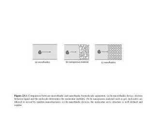
Figure 23.1: Comparison between microfluidic and nanofluidic biomolecule separation. (a) In microfluidic device, friction between liquid and the molecule determines the molecular mobility. (b) In nanoporous material such as gel, molecules are filtered or sieved by random nanostructures. (c) In nanofluidic devices, the molecular sieve structure is well defined and regular.
Figure 23.2: High and Low Reynolds number fluidics. When the Reynolds number is low, viscous interaction between the wall and the fluid is strong, and there is no turbulences or vortices.
Figure 23.3: Hydrodynamic focusing of a liquid stream in a microfluidic channel. Fluid containing fluorescent molecules is driven from the inlet to meet with two other non-fluorescent liquid streams from the side channels. The width of the liquid stream can be controlled by changing the pressures applied to side and inlet channels. In the microchannel, only diffusional mixing can occur, and by narrowing down inlet stream width (wf) one can achieve fast diffusional mixing. (Adapted from Ref. 11 by permission of the American Physical Society.)
Figure 23.4: Charge screening and Debye length. The surface charges are screened by the counterions in the aqueous solution, and the screened charge layer contains mobile, net charges. These mobile charges can drift under the influence of external electric field.
Figure 23.5: Pressure-driven flow vs. Electroosmotic flow. These images were taken by caged dye techniques. At t=0, an initial flat fluorescent line is generated in microchannel by pulse-exposing and breaking the caged dye, rendering them fluorescent. These dyes were transported by the fluid flow generated by pressure-driven flow (left column) or electroosmotic flow (right column), showing the flow profile. (Adapted from P. H. Paul, M. G. Garguilo, and D. J. Rakestraw, Anal. Chem. 70, 2459 (1998) by permission of the American Chemical Society.)
Figure 23.6: Ogston Sieving model. Gel is modeled as a random distribution of fibers in space.
Figure 23.7: Reptation of long polymer (DNA) in gel. (a) Two dimensional schematics of reptation dynamics. Due to the constriction imposed by the gel fibers, the polymer (DNA in this case) can only move along the line of its backbone. (b) Experimental demonstration of reptation-like motion of DNA by Perkins et al. (From Ref. 25 by permission of the American Association for the Advancement of Science.)
Figure 23.8: Steric hindrance effect of globular molecules in nanopores. (a) Schematic diagram demonstrating the steric hindrance effect. The available pore space for the molecule with r will be limited due to the steric hindrance effect. (b) Experimental result by Beck and Schultz. They measured modified (hindered) permeability of molecules with various sizes (0.2 to 2nm) through nanopores with various pore sizes (10~60nm). The ordinate is the hindered diffusion coefficient through the nanopore divided by the free diffusion coefficients in bulk solution. The abscissa is the ratio between molecular and pore radius (2r/d). The solid line represents the Renkin’s calculation. (From Ref. 32 by permission of the American Association for the Advancement of Science.)
Figure 23.9: Scanning electron micrograph of a polymer nanoporous material. The scale bar below is 10 mm. (From Ref. 53 by permission of Wiley Periodicals, Inc.)
Figure 23.10: Two most common method for fabrication of micro /nanofluidic devices. (a) substrate-bonding method (b) sacrificial layer etching method.
Figure 23.11: Pulsed field electrophoresis of long DNA in artificial system. (a) Principles of operation, presented over the optical micrograph of the actual device used. Electric field is switched in direction by 120 degree as shown in the figure. While shorter DNA strand can progress forward, longer DNA strand gets stuck for longer amount of time. After many repetition of this cycle, DNA molecules with different lengths are separated. (b) Separation of two DNA (166kbp and 48kbp) within the system. (From Ref. 69 by permission of the American Chemical Society.)
Figure 23.12: Entropic trap DNA separation. (a) Schematic diagram of entropic trap DNA separation system. (b) Separation result of long DNA molecules. (From Ref. 40 by permission of the American Association for the Advancement of Science.)
Figure 23.13: Nanofluidic Coulter counter for submicrometer particles. (a) Scanning Electron Micrograph of the nanofluidic channel. (b) Detected signal during the passage of several submicrometer particles (bead). (From Ref. 72 by permission of the American Institute of Physics.)
Figure 23.14: Nanopore DNA sequencing. DNA molecules are forced to pass through the nanopore membrane protein, and the current between the two reservoir is monitored. (From Ref. 79 by permission of the Biophysical Society.)
Figure 23.15: Control of electroosmotic flow by external electric field (gate voltage). By applying external potential to the outside surface of a fluidic channel, one can control the electroosmotic flow just as one can control the charge inversion region conductances by controlling gate voltage in MOSFET. (a) normal state. (b) applying negative potential to increase the electroosmotic flow. (c) applying positive potential to decrease or reverse the electroosmotic flow. (From Ref. 18 by permission of the American Association for the Advancement of Science.)
Figure 23.16: FlowFET device fabricated by Schasfoort et al. (a) Schematic diagram of the FlowFET device. The channel wall was 390nm silicon nitride membrane (equivalent to the gate oxide in MOSFET), and external potentials were applied to the gate. (b) Change of electroosmotic flow versus the gate voltage. (From Ref. 18 by permission of the American Association for the Advancement of Science.)