Data Warehousing and Decision Support
Data Warehousing and Decision Support . CS634 Class 22, Apr 28, 2014. Slides based on “Database Management Systems” 3 rd ed , Ramakrishnan and Gehrke , Chapter 25. Introduction.

Data Warehousing and Decision Support
E N D
Presentation Transcript
Data Warehousing and Decision Support CS634Class 22, Apr 28, 2014 • Slides based on “Database Management Systems” 3rded, Ramakrishnan and Gehrke, Chapter 25
Introduction • Increasingly,organizations are analyzing current and historical data to identify useful patterns and support business strategies. • Emphasis is on complex, interactive, exploratory analysis of very large datasets created by integrating data from across all parts of an enterprise; data is fairly static. • Contrast such Data Warehousing and On-Line Analytic Processing (OLAP) with traditional On-line Transaction Processing (OLTP): mostly long queries, instead of the short update Xacts of OLTP. • These are both using “structured data” that can be fairly easily loaded into a database
Structured vs. Unstructured Data • So far, we have been working with structured data • Structured data: • Entities with attributes, each fitting a SQL data type • Relationships • Each row of data is precious • Loads into relational tables, long-term storage • Can be huge • Unstructured data, realm of “big data” • Often doesn’t fit into E/R model, too sloppy • Each piece of data is not precious—it’s statistical • Sometimes just processed and thrown away • No permanent specialized repository, maybe saved in files • Can be really huge
Bigness of Data Big data warehouses, all on Teradata systems See http://gigaom.com/2013/03/27/why-apple-ebay-and-walmart-have-some-of-the-biggest-data-warehouses-youve-ever-seen • Biggest DW: Walmart, passed 1TB in 1992, 2.8 PB (petabytes) = 2800 TB in 2008, growing • eBay: 9 PB DW in 2013, also has 40 PB of big data • Apple: multiple-PB DW • Big data: • Usually over 50TB, can’t fit on one machine • Is judged by “velocity” as well as size • Google: processed 24 PB of data per day in 2009, invented Map-Reduce, published 2004
Teradata • Teradata provides a relational database with ANSI compliant SQL, targeted to data warehouses • Proprietary, expensive ($millions) • Uses a shared-nothing architecture on many independent nodes • Partitioning by rows or (more recently) columns • Scales up well: add node, add network bandwidth for it
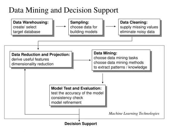
Three Complementary Trends • Data Warehousing: Consolidate data from many sources in one large repository (relational database). • Loading, periodic synchronization of replicas. • Semantic integration, Data cleaning of data on way in • Both simple and complex SQL queries and views. • OLAP: • Complex SQL queries (in effect, but not composed by users). • Queries based on spreadsheet-style operations and “multidimensional” view of data. • Interactive and “online” queries. • Data Mining: Exploratory search for interesting trends and anomalies.
OLAP Data Warehousing EXTERNAL DATA SOURCES • Integrated data spanning long time periods, often augmented with summary information. • Several gigabytes to terabytes common, now petabytes too. • Interactive response times expected for complex queries; ad-hoc updates uncommon. • Read-mostly data EXTRACT TRANSFORM LOAD REFRESH DATA WAREHOUSE Metadata Repository SUPPORTS DATA MINING
Warehousing Issues • Semantic Integration: When getting data from multiple sources, must eliminate mismatches, e.g., different currencies, schemas. • Heterogeneous Sources: Must access data from a variety of source formats and repositories. • Replication capabilities can be exploited here. • Load, Refresh, Purge: Must load data, periodically refresh it, and purge too-old data. • Metadata Management: Must keep track of source (lineage) loading time, and other information for all data in the warehouse.
OLAP: Multidimensional data model • Example: sales data • Dimensions: Product, Location, Time • A measure is a numeric value like sales we want to understand in terms of the dimensions • Example measure: dollar sales value “sales” • Example data point (one row of fact/cube table): • Sales = 25 for pid=1, timeid=1, locid=1 is the sum of sales for that day, in that location, for that product • Pid=1: details in Product table • Locid = 1: details in Location table • Note aggregation here: sum of sales is most detailed data
8 10 10 pid 11 12 13 30 20 50 25 8 15 1 2 3 timeid Multidimensional Data Model timeid sales locid pid • SalesCube(pid, timeid, locid, sales) • Collection of numeric measures, which depend on a set of dimensions. • E.g., measure sales, dimensions Product (key: pid), Location (locid), and Time (timeid). • Full table, pg. 851 Slice locid=1 is shown: locid
Granularity of Data • Example of last slide uses time at granularity of days • Individual transactions (sales at cashier) have been added together to make one row in this table • Note: “measures” can always be aggregated • Current hardware can handle more data • Typical data warehouses hold the original transaction data • So such a fact table has more columns, for example • dateid, timeofday, prodid, storeid, txnid, clerkid, sales, …
Data Warehouse vs. Data for OLAP • Current DW fact table is huge, with individual transactions, large number of dimensions • Can only use a subset of this for OLAP, because of explosion of cells • Take DW fact table, roll up to days (say), drop less important columns, get much smaller data for OLAP • Load data into OLAP, another tool. • Table on pg. 851 is a cube table, not a DW fact table • Can think of OLAP as a cache of most important aggregates of DW tables
MOLAP vs ROLAP vs HOLAP • Multidimensional data can be stored physically in a (disk-resident, persistent) array; called MOLAP systems. Alternatively, can store as a relation; called ROLAP systems; • hybrid of these = HOLAP, current systems • The main relation, which relates dimensions to a measure, is called the fact table. Each dimension can have additional attributes and an associated dimension table. • E.g., Products(pid, pname, category,price ) • Fact tables are much larger than dimensional tables.
Dimension Hierarchies: OLAP, DW • For each dimension, the set of values can be organized in a hierarchy: PRODUCT TIME LOCATION year quarter country category week month state pname date city
Schema underlying OLAP, used in DW TIMES • Fact/cube table in BCNF; dimension tables not normalized. • Dimension tables are small; updates/inserts/deletes are rare. So, anomalies less important than good query performance. • This kind of schema is very common in DW and OLAP, and is called a star schema; computing the join of all these relations is called a star join. • Note: in OLAP, this is not what the user sees, it’s hidden underneath • In DW, this is the basic setup, but usually with more dimensions • Here only one measure, sales, but can have several timeid date week month quarter year holiday_flag (Fact table) pid timeid locid sales SALES PRODUCTS LOCATIONS pid pname category price locid city state country
OLAP (and DW) Queries • Influenced by SQL and by spreadsheets. • A common operation is to aggregate a measure over one or more dimensions. • Find total sales. • Find total sales for each city, or for each state. • Find top five products ranked by total sales. • Roll-up: Aggregating at different levels of a dimension hierarchy. • E.g., Given total sales by city, we can roll-up to get sales by state.
OLAP Queries • Drill-down: The inverse of roll-up: go from sum to details that were added up before • E.g., Given total sales by state, can drill-down to get total sales by county. • Drill down again, see total sales by city • E.g., Can also drill-down on different dimension to get total sales by product for each state.
OLAP Queries: cross-tabs With relational DBs, we are used to tables with column names across the top, rows of data. With OLAP, a spreadsheet-like representation is common, Called a cross-tabulation: • One dimension horizontally • Another vertically WI CA Total 63 81 144 1995 38 107 145 1996 75 35 110 1997 176 223 339 Total
OLAP Queries: Pivoting WI CA Total • Example cross-tabulation: • Pivoting: switching dimensions on axes, or choosing what dimensions to show on axes • Switching dimensions means pivoting around a point in the upper-left-hand corner • End up with “1995 1996 1997 Total” across top, • “WI CA Total” down the side 63 81 144 1995 38 107 145 1996 75 35 110 1997 176 223 339 Total
Oracle 11 supports cross-tabs display select * from ( select times_purchased, state_code from customers t ) pivot ( count(state_code) for state_code in ('NY','CT','NJ','FL','MO') ) order by times_purchased Here is the output: TIMES_PURCHASED 'NY' 'CT‘ 'NJ' 'FL‘ 'MO' --------------- ---------- ---------- ---------- ---------- -- 0 16601 90 0 0 0 1 33048 165 0 0 0 2 33151 179 0 0 0 3 32978 173 0 0 0 4 33109 173 0 1 0 ... and so on ... (We have Oracle 10, unfortunately)
SQL Queries for cross-tab entries WI CA Total 63 81 144 1995 The cross-tabulation values can be computed using a collection of SQL queries: 38 107 145 1996 75 35 110 1997 176 223 339 Total SELECT SUM(S.sales) FROM Sales S, Times T, Locations L WHERE S.timeid=T.timeid AND S.timeid=L.timeid GROUP BYT.year, L.state SELECT SUM(S.sales) FROM Sales S, Times T WHERE S.timeid=T.timeid GROUP BYT.year SELECT SUM(S.sales) FROM Sales S, Location L WHERE S.timeid=L.timeid GROUP BY L.state
The CUBE Operator • Generalizing the previous example, if there are k dimensions, we have 2^k possible SQL GROUP BY queries that can be generated through pivoting on a subset of dimensions. • CUBE Query, pg. 857 • Equivalent to rolling up Sales on all eight subsets of the set {pid, locid, timeid}; each roll-up corresponds to an SQL query of the form: SELECT T.year, L.state, SUM(S.sales) FROM Sales S, Times T, Locations L WHERES.timeid = T.timeid and S.locid = L.locid GROUP BY CUBE (T.year, L.state) SELECT SUM(S.sales) FROM Sales S GROUP BY grouping-list
Oracle 10 supports CUBE queries select t.year, s.store_state, sum(dollar_sales) from salesfact f, times t, store s where f.time_key = t.time_key and s.store_key = f.store_key group by cube(t.year, s.store_state); YEAR STORE_STATE SUM(DOLLAR_SALES) ---------- -------------------- ----------------- 781403.59 AZ 35684 CA 77420.82 CO 38335.26 (some rows deleted) TX 40886.54 WA 39540.16 1994 396355.76 1994 AZ 17903.04 1994 CA 38966.54 1994 CO 17870.33 1994 DC 20901.18 … from dbs2 output
DW data OLAP • The CUBE query can do the roll-ups on DW data needed for OLAP
Excel is the champ at OLAP queries • Next time will do Excel pivot table demo • Based on video by Minder Chen of UCI (Cal state U/Channel Islands) • https://www.youtube.com/watch?v=eGhjklYyv6Y • Setup: • His MS Access database with star schema for sales • Create view of fact joined with desired dimension data (a star join) • Point Excel at this big view, ask it to create pivot table • Pivot table: drill down, roll up, pivot, …
Excel can use Oracle data too • The database from Chen’s demo is now in dbs2’s Oracle • We could point Excel to an Oracle view of joined tables. • How does that work? • Use ODBC (Open Database Connectivity), older than JDBC, but roughly same idea • Provides client API for accessing multiple databases • Each database provides a ODBC driver • Unfortunately, it’s not easy to set up ODBC on a Windows system even though Microsoft invented it
Star queries • Oracle definition: a query that joins a large (fact) table to a number of small (dimension) tables, with provided WHERE predicates on the dimension tables to reduce the result set to a very small percentage of the fact table • The select list still has sum(sales), etc., as desired. SELECT store.sales_district, time.fiscal_period, SUM(sales.dollar_sales) FROM sales, store, time WHERE sales.store_key = store.store_key AND sales.time_key = time.time_key AND store.sales_district IN ('San Francisco', 'Los Angeles') AND time.fiscal_period IN ('3Q95', '4Q95', '1Q96') GROUP BY store.sales_district,time.fiscal_period;
Star queries • Oracle: A better way to write the query would be: (i.e., give the QP a hint on how to do it) SELECT ... FROM sales WHERE store_key IN ( SELECT store_key FROM store WHERE sales_district IN ('WEST', 'SOUTHWEST')) AND time_key IN ( SELECT time_key FROM time WHERE quarter IN ('3Q96', '4Q96', '1Q97')) AND product_key IN ( SELECT product_key FROM product WHERE department = 'GROCERY') GROUP BY …; • Oracle will rewrite the query this way if you add the STAR_TRANSFORMATION hint to your SQL, or the DBA has set STAR_TRANSFORMATION_ENABLED
Excel can do Star queries • Recall GROUP BY queries for individual crosstab entries • A Star query is of this form, plus WHERE clause predicates on dimension tables such as • store.sales_district IN ('WEST', 'SOUTHWEST') • time.quarter IN ('3Q96', '4Q96', '1Q97') • Excel allows “filters” on data that correspond to these predicates of the WHERE clause
Indexes related to data warehousing • New indexing techniques: Bitmap indexes, Join indexes, array representations, compression, precomputation of aggregations, etc. • E.g., Bitmap index: sex custid name sex rating rating Bit-vector: 1 bit for each possible value. Many queries can be answered using bit-vector ops! F M
Bitmap Indexes • A bitmap index uses one bit vector (BV) for each distinct keyval • The number of bits = #rows • Example of last slide, 4 rows, 2 columns with bitmap indexes • Sex = ‘M’: BV = 1101 • Sex = ‘F’: BV = 0010 • Rating = 3, BV = 1000 • Rating = 4, BV = 0001 • Rating = 5, BV = 0110 Bitmap index for sex column Bitmap index for rating column
Bitmap Indexes • Implementation: B+-tree of key values, bitmap for each key • Size = #values*#rows/8 if not compressed • Bitmaps can be compressed, done by Oracle and others • Main restriction: slow row insert/delete, so NG for OLTP • But great for data warehouses: • Data warehouses are updated only periodically, traditionally • Low cardinality (#values in column) a clear fit • Example: rating, with 10 values • But in fact, cardinality can be fairly high with compression • Oracle example: bitmap index on unique column!
Bitmap Indexes • Oracle: create bitmap index sexx on custs(sex); • Bitmap indexes can be used with AND and OR predicates • Example Select name from sailors s where s.rating = 10 and sex = ‘M’ or sex = ‘F’ BV1 BV2 BV3 ResultBV = BV1 & BV2 | BV3 • Each bit on in ResultBV shows a row that satisfies the predicate • Loop through on-bits, finding rows and output name
Oracle Bitmap index plan • EXPLAIN PLAN FOR SELECT * FROM t WHERE c1 = 2 AND c2 <> 6 OR c3 BETWEEN 10 AND 20; • EXPLAIN PLAN FOR • SELECT * FROM t WHERE c1 = 2 AND c2 <> 6 OR c3 BETWEEN 10 AND 20; • SELECT STATEMENT • TABLE ACCESS T BY INDEX ROWID • BITMAP CONVERSION TO ROWID -- get ROWIDs for each on-bit • BITMAP OR --top level OR • BITMAP MINUS --to remove null values of c2 • BITMAP MINUS -- to calc c1 = 2 AND c2 <> 6 • BITMAP INDEX C1_IND SINGLE VALUE --c1= 2 BV • BITMAP INDEX C2_IND SINGLE VALUE --c2 = 6 BV • BITMAP INDEX C2_IND SINGLE VALUE --c2 = null BV (no not null on col) • BITMAP MERGE --merge BV’s over C3 range • BITMAP INDEX C3_IND RANGE SCAN
Bitmaps for star schemas, to be continued • The dimension tables are not large, maybe 100 rows • Thus the FK columns in the fact table have only 100 values • Bitmap indexes can pinpoint rows once determined. • Bitmaps can be AND’d and OR’d • Example: time.fiscal_period IN ('3Q95', '4Q95') matches say 180 days in time table, so 180 FK values in fact’s time_key column • OR together the 180 bitmaps, get a bitmap locating all fact rows that satisfy this predicate