Download
1 / 12
350 likes | 1.38k Views
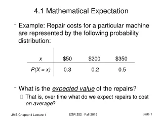
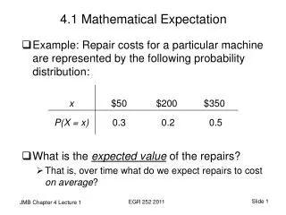
4.1 Mathematical Expectation. Example: Repair costs for a particular machine are represented by the following probability distribution: What is the expected value of the repairs? That is, over time what do we expect repairs to cost on average ?. Expected Value – Repair Costs.

E N D
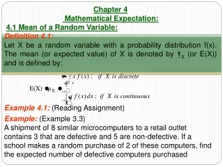
4.1 Mathematical Expectation • Example: Repair costs for a particular machine are represented by the following probability distribution: • What is the expected value of the repairs? • That is, over time what do we expect repairs to cost on average? EGR 252 2011
Expected Value – Repair Costs • μ = E(X) • μ= mean of the probability distribution • For discrete variables, μ = E(X) = ∑ x f(x) So, for our example, • E(X) = 50(0.3) + 200(0.2) + 350(0.5) = $230 EGR 252 2011
Another Example – Investment • By investing in a particular stock, a person can take a profit in a given year of $4000 with a probability of 0.3 or take a loss of $1000 with a probability of 0.7. What is the investor’s expected gain on the stock? X $4000 -$1000 P(X) 0.3 0.7 E(X) = $4000 (0.3) -$1000(0.7) = $500 EGR 252 2011
Expected Value - Continuous Variables • For continuous variables, μ = E(X) = E(X) = ∫ x f(x) dx • Vacuum cleaner example: problem 7 pg. 88 x, 0 < x < 1 f(x) = 2-x, 1 ≤ x < 2 0, elsewhere (in hundreds of hours.) { = 1 * 100 = 100.0 hours of operation annually, on average EGR 252 2011
Functions of Random Variables • Ex 4.4. pg. 111: Probability of X, the number of cars passing through a car wash in one hour on a sunny Friday afternoon, is given by • Let g(X) = 2X -1 represent the amount of money paid to the attendant by the manager. What can the attendant expect to earn during this hour on any given sunny Friday afternoon? E[g(X)] =Σg(x) f(x) = Σ (2X-1) f(x) = (2*4-1)(1/12) +(2*5-1)(1/12) …+(2*9-1)(1/6) = $12.67 EGR 252 2011
4.2 Variance of a Random Variable • Recall our example: Repair costs for a particular machine are represented by the following probability distribution: • What is the variance of the repair cost? • That is, how might we quantify the spread of costs? EGR 252 2011
Variance – Discrete Variables • For discrete variables, • σ2 = E [(X - μ)2] = ∑ (x - μ)2 f(x) = E (X2) - μ2 • Recall, for our example, μ = E(X) = $230 • Preferred method of calculation: • σ2 = [E(X2)] – μ2 = 502 (0.3) + 2002 (0.2) + 3502 (0.5) – 2302 = $17,100 • Alternate method of calculation: • σ2 = E(X- μ)2 f(x) = (50-230)2 (0.3) + (200-230)2 (0.2) + (350-230)2 (0.5) = $17,100 EGR 252 2011
Variance - Investment Example • By investing in a particular stock, a person can take a profit in a given year of $4000 with a probability of 0.3 or take a loss of $1000 with a probability of 0.7. What are the variance and standard deviation of the investor’s gain on the stock? • E(X) = $4000 (0.3) -$1000 (0.7) = $500 • σ2 = [∑(x2 f(x))] – μ2 = (4000)2(0.3) + (-1000)2(0.7) – 5002 = $5,250,000 • σ = $2291.29 EGR 252 2011
Variance of Continuous Variables • For continuous variables, σ2 = E [(X - μ)2] =[∫ x2 f(x) dx] – μ2 • Recall our vacuum cleaner example pr. 7 pg. 88 x, 0 < x < 1 f(x) = 2-x, 1 ≤ x < 2 0, elsewhere (in hundreds of hours of operation.) • What is the variance of X? The variable is continuous, therefore we will need to evaluate the integral. { EGR 252 2011
Variance Calculations for Continuous Variables • (Preferred calculation) • What is the standard deviation? • σ = 0.4082 hours EGR 252 2011
Covariance/ Correlation • A measure of the nature of the association between two variables • Describes a potential linear relationship • Positive relationship • Large values of X result in large values of Y • Negative relationship • Large values of X result in small values of Y • “Manual” calculations are based on the joint probability distributions • Statistical software is often used to calculate the sample correlation coefficient (r) EGR 252 2011
What if the distribution is unknown? • Chebyshev’s theorem: The probability that any random variable X will assume a value within k standard deviations of the mean is at least 1 – 1/k2. That is, P(μ – kσ < X < μ + kσ) ≥ 1 – 1/k2 • “Distribution-free” theorem – results are weak • If we believe we “know” the distribution, we do not use Chebyshev’s theorem to characterize variability EGR 252 2011