Analyzing Ocean Profiles: T, S, p Along 150W from 45S to 45N
Explore seasonal ocean profiles of temperature, salinity, and pressure along 150W from 45S to 45N using Levitus data. Utilize Seawater routines for computations and contour plots. Focus on upper 1500m and examine temporal variability. Enhance your understanding of acoustical oceanography and sound propagation by diving into the lecture topics on wave physics and more.

Analyzing Ocean Profiles: T, S, p Along 150W from 45S to 45N
E N D
Presentation Transcript
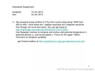
Homework Assignment • assigned: 10 Jan 2013 • due: 22 Jan 2013 • Get seasonal ocean profiles of T,S,p from Levitus data along 150W from 45S to 45N. I think these are 1 degree resolution but 5 degrees would be fine (though not much less work). You can get these at http://ingrid.ldgo.columbia.edu/SOURCES/.LEVITUS94/. Use Seawater routines to compute and contour plot potential temperature , potential density , and sound speed, c. Focus on the upper 1500m. Comment on temporal variability. get Oceans toolbox at http://woodshole.er.usgs.gov/operations/sea-mat/ Oc679 Acoustical Oceanography
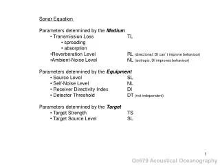
Next few lectures: Lighthill Ch.1 Medwin&Clay Ch.2 Wave physics acoustic intensity / pressure spreading / reflection / refraction ( propagation properties ) interference ( “near-field” effects ) definition of the “far-field” wave properties the wave equation acoustic impedance reflection / transmission … quantified some properties head waves Doppler sonar Sonar Equation define unit of measurement for acoustics absorption transmission losses example tomography
Physics of Sound Propagation – M&C Ch2 sound is a mechanical disturbance travels as longitudinal or compressive wave (in geophysics, P-wave) (compared to a transverse wave – like surface gravity waves) transverse/longitudinal wave applet identified as an incremental acoustic pressure << ambient pressure In a homogenous, isotropic medium, an explosion will create adjacent region of higher density, pressure – condensation pulse By contrast, rarefaction pulse created by implosion This pulse will move away as a spherical wave shell so that the initial energy is spread over shells of larger radii, but lower intensity - spherical spreading absorption and scattering affect intensity Oc679 Acoustical Oceanography
acoustic wavelengths f=c/f 10 Hz 150 m 100 Hz 15 m 1 kHz 1.5 m 10 kHz 15 cm 100 kHz 1.5 cm 1 MHz 1.5 mm 10 MHz 150 m 100 MHz 15 m
p, acoustic pressure (unit [Pa]) pA = ρgh + atmospheric pressure + waves + nonhydrostatic effects time sound pressure sound silence pA, total ambient pressure (unit [Pa]) 1 m water ≈ 104 Pa atmospheric pressure ≈ 105 Pa large amplitude internal wave ≈ 100 Pa fin whale (100 m range) ≈ 10 Pa ATOC source level (75 Hz) ≈ 104 Pa (200 dB) total pressure 0
spherical spreading Acoustic intensity = energy per unit time passing thru a unit surface area [J s-1 m-2] Total energy is integrated over spherical surface 4πR2 Conservation of energy 4πR2·iR = 4πR02·i0 iR, io are acoustic intensities at R, Ro pulse has duration t Therefore, Sound intensity decreases as 1/R2 – this is termed spherical spreading Oc679 Acoustical Oceanography
Modifications to wave propagation • Reflection – wave incident on boundary • Refraction – change in sound speed changes direction of wave propagation as well • Interference – combination of sound waves – phase-dependent • Diffraction – when sound encounters an obstacle some of the energy bends around it, some is reflected Oc679 Acoustical Oceanography
Huygens’ principle –useful for geometrical construction of reflection, refraction and diffraction Consider each point on an advancing front as a source of secondary waves, each moving outward as spherical wavelets – the outer surface that envelops these waves represents the new wave front In timet, wavelets originating at wave front a, travel R to b, which is now the location of the new wave front Oc679 Acoustical Oceanography
Law of reflection: angle of reflection of rays ( wave fronts) = angle of incidence, and is in the same plane Law of refraction (Snell’s Law): where 1, 2 are angles measured between rays and normal to interface or between wave fronts and interface c1, c2 are the sounds speeds in the 2 media M&C (fig 2.2.3) show a sketch of the case c2>c1 Huygens’ principle demonstrates laws of reflection and refraction reflection/refraction applet http://webphysics.ph.msstate.edu/jc/library/24-2/huygens.htm Oc679 Acoustical Oceanography
wave refraction which is greater c1? or c2?
wave refraction you can tell this by considering that frequency is invariant f = c1/λ1 = c2/λ2 = constant c1 > c2 rays bend towards lower c medium
applet example – waves had traveled from a distant point such that wave curvature was negligible (plane wave approximation) below is a spherical wave reflected wave fronts point source above a half-plane reflected wave fronts appear to come from an image source in lower half-plane Oc679 Acoustical Oceanography
sound speed profile refracted / refracted refracted / surface-reflected surface-reflected / bottom-reflected these are computed from ray theory – integration of odes initial condition is the ray take-off angle this figure shows the paths from many take-off angles
sound propagation paths in the ocean c(z) c(z)
sound propagation paths in the ocean nearly isothermal stratified c(z) c(z)
sound propagation paths in the ocean c(z) c(z)
single slit diffraction radially-spreading wave from a plane wave
Diffraction – obstacle effects http://www.phy.hk/wiki/englishhtm/Diffraction2.htm obstacle Oc679 Acoustical Oceanography
Interference effects Phase fT [cycles], 2fT [radians] temporal phase 2R/ [radians] spatial phase interference effects from local source / source array may be important in the near-field of the source
Interference effects interference effects from local source / source array may be important in the near-field of the source 192 element array Urick Fig 3.3 near-field of an ultrasonic transducer http://www.ndt-ed.org/EducationResources/CommunityCollege/Ultrasonics/EquipmentTrans/radiatedfields.htm
Interference effects Lloyd’s Mirror Effect (optics) has an analogue in underwater acoustics (surface interference effect) this is a straightforward case of interference of acoustic signals in which one of the sources is the surface reflection of the source wave the result is an interference pattern with peaks and troughs in signal intensity along range R. Ultimately, I decreases as 1/R2. 2.4.2 – 2.4.4 (M&C) Oc679 Acoustical Oceanography
Newton’s 2nd Law for Acoustics F = ma pressure across a fluid CV thru which acoustic wave travels applies at point x and time t [w1] rate at which CV is accelerated Sound Wave Physics we consider a small region far from an oscillating spherical source where plane wave approximation holds - direction of propagation is x or R subscript Arefers to the ambient pressure, density, which are constant p, are acoustic pressure, density so p, du/dt in quadrature p,u out of phase by π Conservation of Mass for Acoustics Here the compressibility of the fluid, however small, is important – more mass can flow into a CV than out, resulting in a net density change in the CV [w2] Oc679 Acoustical Oceanography
Equation of State for Acoustics Hooke’s law for an elastic body stress strain force per unit area relative change in dimension • For acoustics • stress is the acoustic pressure, p • strain is the relative change of density, /A • proportionality constant is bulk modulus of elasticity, E • this is equivalent to an acoustical equation of state [w3] 1D wave equation Eliminating u in [w1, w2] and using w3, we get the 1D linear acoustic wave equation [w4] alternatively, we could have eliminated p rather than using [w3] and obtained an equation for the acoustic density This can be derived for the particle velocity, u, or particle displacement or other parameters characteristic of the wave - p used as hydrophones are pressure-sensitive Oc679 Acoustical Oceanography
recall (remember ) property of the medium property of the wave wave equation has solutions of form substituting plane wave solution into wave equation gives [w5] so we can write the wave equation as acoustic impedance this is shown by substitution satisfy plane waves of form substitution into [w1] integrating w.r.t. x note resemblance to Ohm’s law V = ZI where V is voltage, Z is impedance and I is current Ac, or rho-c is the acoustic impedance and is a property of the material Oc679 Acoustical Oceanography
acoustic Mach number from [w2] and can determine ratio of acoustic particle velocity to sound speed where M is a kind-of Mach number, a measure of the strength of the sound wave and thereby the linearity of the signal propagation – interesting and important effects for high M acoustic pressure-density relation combining and c=√p/ρ this means that c can be computed from an equation of state for seawater c=c(S,T,p) [this is included in seawater routines] http://sea-mat.whoi.edu/ Oc679 Acoustical Oceanography
( ) acoustic intensity defined as the energy per unit time [ power ] - passing through a unit area a wave traveling in the +x direction has intensity defined by the product of the instantaneous values of acoustic pressure and the particle velocity - since c is not a function of direction, no subscript x needed note: units are W/m2 using the equation for acoustic impedance with the long range plane wave approximation (replace x with R) for a sinusoidal wave instantaneous intensity ixoscillates between 0 and P2/(Ac) at frequency 2 average intensity - time average at x note: analogy to electronics in which Power = V2/Z this is alternatively U2 via acoustic impedance equation where P is peak pressure, P=2Prms Oc679 Acoustical Oceanography
summary – sound wave physics property of the medium property of the wave conservation of momentum 1-D wave equation conservation of mass solutions acoustical equation of state c=√p/ρ rho-c is acoustic impedance or relationship of c to properties of the medium average acoustic intensity 31
Reflection and Transmission at interfaces • plane waves • boundary conditions • pressures equal on each side of interface • normal components of particle velocity equal on each side of interface ui ur ut normal components of particle velocity are replacing u with p using acoustic impedance relationship Oc679 Acoustical Oceanography
define reflection and transmission coefficients pressure boundary condition velocity boundary condition these boundary conditions give the pressure reflection and transmission coefficients in terms of the angles of incidence & refraction and density and sound speeds in the media on each side of the interface example source beneath water-air interface which is unrealistically smooth is normally incident to the interface (cos1=1, cos2=1) air1 kg/m3, cair 330 m/s,water1000 kg/m3, cwater 1500m/s so that 1c1 2c2, T12 0, R12 -1 (the negative sign indicates phase – incident and reflected pressures out of phase – since wave speeds are in opposite direction) (this is an example of total reflection due to impedance mismatch) [what happens when 1c1= 2c2?] perfect transmission when 1c1= 2c2 Oc679 Acoustical Oceanography
we can also get total reflection for sufficiently large incident angles into higher c medium Snell’s law can be written and R12 Snell’s law gives use sin2+cos2 =1 when cos2 is complex this occurs when where subscript c refers to a critical angle when 1 < c, R12 is real and |R12| < 1 (lossy medium) when 1 > c, R12 is imaginary and |R12| = 1 but with a phase shift given by 1=1033 kg/m3 c1=1508 m/s 2=2 1 c2=1.12c1 if one is interested in getting acoustic signal across the interface (i.e., across the bottom sediments), R12 is a bottom loss Oc679 Acoustical Oceanography
water sediments bedrock Reflection and Transmission at multiple thin layers where layer thicknesses small compared to distances to source/receiver, can use plane wave assumption the net return signal is the sum of the reflection/transmission coefficients in the layers, with proper inclusion of the phase delay of the vertical wavenumber component through each layer i=kwavehicosI, where hi is layer thickness M&C section 2.6.3 an example of where this analysis might be used is shown here – bottom layers are identified by the reflections at different depths (source/receiver is 3 m below water surface – transmitted signal is 1 cycle of a 7 kHz sinusoid) 0 m using c = 1500m/s we can convert time scale to range or depth scale (at least to the seafloor, below which c >> 1500) range = ct/2 t is the total travel time from source back to receiver 37.5 m 2nd reflection Oc679 Acoustical Oceanography
Head waves • we now consider spherical waves propagating into a higher speed medium adjacent to the source medium • head wave moves at higher speed c2 along the interface and radiate into source medium • at sufficiently large ranges it will arrive ahead of the direct wave • rays propagate into source medium at critical angle given by sinc=c1/c2 what happens at angles < c? weak reflection at steep angles angle = c ? this is the angle the ray path must take to make θ2=90° angles > c? pure reflection, no transmission properties can be deduced by Huygens wavelets construction here c2=2c1, c=30 at angles > csound pressures and displacements are equal on both sides of interface and are excited at points hi moving as the refracted wave along the interface at c2 the head wave front is the envelope of the wavelets for a spherical point source, head wave is represented by a conical surface in 3D Oc679 Acoustical Oceanography
axial arrivals short path at low speed less attenuation due to cylindrical spreading no reflective losses interfering reflected arrivals long path length at high speed attenuated by reflection at top/bottom head wave what does an arrival look like? Oc679 Acoustical Oceanography
spherical wave (D) – pulse has yet to contact surface • pulse has met interface – reflected (R) and transmitted (T) waves apparent – • notes: • T has longer pulse length due to higher c • R shows critical angle effect of reduced amplitude for steep angles (earlier arrivals at interface) T has pulled ahead of D, R head wave is 1st arrival near interface, but further away, direct wave arrives 1st note scale change Oc679 Acoustical Oceanography source: Computational Ocean Acoustics
following is a simulation of acoustic waves traveling outward from the source, reflecting from a higher-velocity material below and from the free surface above c1=6000 m/s c2=8000 m/s Oc679 Acoustical Oceanography
change of phase upon reflection at free surface source Oc679 Acoustical Oceanography
The next animation shows the same model, but looking at greater distances and later times. In this case, the refracted wave in the lower medium is clear, the head wave can be seen to develop with a cross-over distance of about 120 km. The linearity of the head wave as it propagates upward is particularly well illustrated by the animation. There is a weak numerical artifact (which appears as a wave propagating up from the bottom of the image) due to not-quite absorbing boundary conditions. The amplitudes in this figure are greatly enhanced so that the head wave is visible; unfortunately, so are the numerical errors. Once again, click on the still image to view the animation http://www.geol.binghamton.edu/~barker/animations.html Oc679 Acoustical Oceanography
axial arrivals short path at low speed less attenuation due to cylindrical spreading no reflective losses interfering reflected arrivals long path length at high speed attenuated by reflection at top/bottom head wave what does an arrival look like? Oc679 Acoustical Oceanography
summary – sound wave physics property of the medium property of the wave conservation of momentum 1-D wave equation conservation of mass solutions acoustical equation of state c=√p/ρ rho-c is acoustic impedance or relationship of c to properties of the medium average acoustic intensity
. . . . . . . . . . . . . . . . . . . . . fsource transducer V fsource+fDoppler Doppler sonar such as an ADCP (acoustic Doppler current profiler) measure of the velocity of water from the shift in frequency of a transmitted pulse wavelength of the traveling wave is constant λDoppler = λsource so fDoppler= - fsource(V/c)fDoppler = change in returned frequency fsource = frequency of transmitted signal V = velocity of scatterers c = sound speed operation of a monostatic ADCP, or a transducer (transceiver) that generates a short pulse at fsource which propagates through the water. Signal is transmitted in all directions by small scatterers (smaller than the acoustic wavelength) – some fraction is reflected back along beam axis – ADCP senses signal with a modulated frequency fsource+fDoppler Oc679 Acoustical Oceanography
acoustic travel time measurement t1 = R/c t1 = R/c + R/U source/ receiver source/ receiver receiver/ reflector receiver/ reflector t2 = R/c t2 = R/c –R/U what can we learn from a source/receiver pair? separated by range R in medium with sound speed c if U = 0, sound speed c is determined by measuring t1 or t2 t1 = R/c, t2 = R/c, t1 + t2 = 2R/c U if U 0 t1 + t2 = 2R/c t1 - t2 = 2R/U Oc679 Acoustical Oceanography
Continuous wave sinusoidal signals Wavelength, is the distance between adjacent condensations (or adjacent rarefactions) along direction of travel of wavefront Radiation from a small sinusoidal source I just wrote this down here. It is not obvious but it is a consequence of conservation of energy At a point, time between adjacent condensations, T = /c = 1/f or c = f here T [s], f [Hz], [m], c [m/s] Dimensionless products fT [cycles], 2fT [radians] temporal phase compare 2R/ spatial phase Radian frequency, = 2f = 2/T [rad/s] Wavenumber, k = 2/ [rad/m] c = /k Oc679 Acoustical Oceanography