Download
1 / 1
10 likes | 82 Views
Explore a method utilizing digital filters for real-time reconstruction of signals affected by high-frequency noise, demonstrated with temperature profiles from Vaisala Sensor data. Understand how slow sensor responses can be overcome to improve data accuracy and efficiency.

E N D
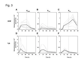
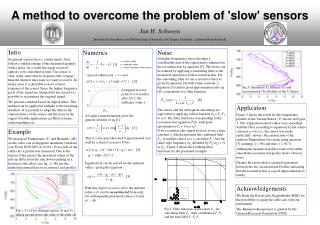
Numerics Noise At higher frequencies noise becomes a considerable part of the signal and is enhanced in the reconstruction by equation [5]. This noise can be reduced by applying a smoothing filter to the measured signal prior to the reconstruction. For the smoothing filter we use a recursive filter as given by equation [4] with a time constant f. Equation [3] (and in good approximation also eq. [4]) corresponds to a filter function y = sensor value x = ambient value s = time constant of the sensor special solution for x = const. : Fig.3: measured (T), filtered (Tf) and reconstructed (Tx) Profiles of the V Sensor A tangent at every point of y(t) reaches after t=s the ambiance value x x y0 The sensor and the subsequent smoothing are equivalent to applying a filter function Ffs= Fs·Ff to x(t). The filter function corresponding to the reconstruction equation [5] is with good aproximation Fx = 1+(x)2. If we reconstruct the signal we have to use a time constant x which represents the combined filter Ffs. A suitable choice is a x such that Fx-1 has the same edge frequency ½ definded by Fx(½) = ½ as Ffs. Figure 2 shows the resulting filter functions for the presented example. t/s A Laplace transformationgives the general solution of eq.[1]: This is a low pass filter and is aproximated very well by a digital recursive Filter: Equation [4] can be solved for the ambient value x giving the equation With this digital recursive filter the ambient values x(t) can be reconstructedfrom only two subsequently measured values y(t) and y(tt). Fig.2: Filter functions of the sensor Fs, the smoothing filter Ff , their combination Fs·Ff and the final filter Fs·Ff·Fx Fig.1: T vs P for different sensors (F and V) during up and down (dn) rides of the cable car A method to overcome the problem of 'slow' sensorsJan H. SchweenInstitute for Geophysics and Meteorology, University of Cologne, Germany , jschween@uni-koeln.de Intro In general sensors have a certain inertia, they follow a sudden change of the measured quantity with a delay. As a result the signal received appears to be smoothed in time. The sensor is slow in the sense that its response time is larger than the shortest time scale we want to resolve. In many cases it is desirable to have a faster response of the sensor. Since the higher frequency parts of the signal are damped but not erased it is possible to reconstruct the original signal. We present a method based on digital filters. This method can be applied in realtime to the incoming dataflow. It is possible to adapt the filter to the characteristics of the sensor and the noise in the signal. Possible applications are REA systems, radiosoundings etc. Application Figure 3 shows the result for the temperature profiles of the Vaisala Sensor (V) shown in Figure 1. The original measured values were smoothed with the filter according to equation [4] and a time constant f = 6s (i.e. the sensor was made artificially slower). Reconstruction of the ambient Temperature was made using equation [5] asuming s = 50s and thus x = 50.7s. Althoug the measured profiles seem to be rather smooth the reconstructed profile shows obvious noise. Despite this noise there is general agreement between the two reconstructed Profiles indicating that the reconstruction is a good approximation to reality. Example We measured Temperature (T) and Humidity (rH) on the cable cars at Zugspitze mountain, Germany (see Poster EGU2007-A-10161). Every ride of the cable cars a profile was measured. Due to the inertia of the sensors the measured values of the ride up differ from the ride down resulting in a hysteresis like effect (see fig. 1). We use the method presented here to reconstruct real profiles. Acknowledgements We thank the Bayerische Zugspitzbahn (BZB) for the possibility to equip the cable cars with our instruments. The Bannerwolken project is granted by the German Research Foundation (DFG)