Discrete Distributions
Discrete Distributions What is the binomial distribution? The binomial distribution is a discrete probability distribution. It is a distribution that governs the random variable, X, which is the number of successes that occur in " n" trials.


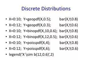
Discrete Distributions
E N D
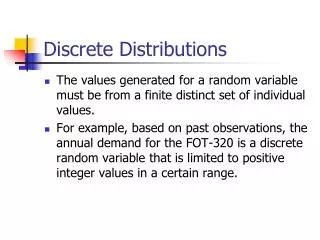
Presentation Transcript
What is the binomial distribution? The binomial distribution is a discrete probability distribution. It is a distribution that governs the random variable, X, which is the number of successes that occur in "n" trials. The binomial probability distribution gives us the probability that a success will occur x times in the n trials, for x = 0, 1, 2, …, n. Thus, there are only two possible outcomes. It is conventional to apply the generic labels "success" and "failure" to the two possible outcomes. Discrete Distributions
A success can be defined as anything! "the axle failed" could be the definition of success in an experiment testing the strength of truck axles. Examples: 1.A coin flip can be either heads or tails 2.A product is either good or defective Binomial experiments of interest usually involve several repetitions or trials of the same basic experiments. These trials must satisfy the conditions outlined below: Discrete Distributions
When can we use it? Condition for use: Each repetition of the experiment (trial) can result in only one of two possible outcomes, a success or failure. See example BD1. The probability of a success, p, and failure (1-p) is constant from trial to trial. All trials are statistically independent; i.e. No trial outcome has any effect on any other trial outcome. The number of trials, n, is specified constant (stated before the experiment begins). Discrete Distributions
Example 1: binomial distribution: A coin flip results in a heads or tails A product is defective or not A customer is male or female Example 4: binomial distribution: Say we perform an experiment – flip a coin 10 times and observe the result. A successful flip is designated as heads. Assuming the coin is fair, the probability of success is .5 for each of the 10 trials, thus each trial is independent. We want to know the number of successes (heads) in 10 trials. The random variable that records the number of successes is called the binomial random variable. Random variable, x, the number of successes that occur in the n = 10 trials. Discrete Distributions
Do the 4 conditions of use hold? We are not concerned with sequence with the binomial. We could have several successes or failures in a row. Since each experiment is independent, sequence is not important. The binomial random variable counts the number of successes in n trials of the binomial experiment. By definition, this is a discrete random variable. Binomial Random Variable
Calculating the Binomial Probability • Rather than working out the binomial probabilities from scratch each time, we can use a general formula. • Say random variable "X" is the number of successes that occur in "n" trials. • Say p = probability of success in any trial • Say q = probability failure in any trial where q = (1 – p) • In general, The binomial probability is calculated by: Where x = 0, 1, 2, …, n
Example: For n = 3 Calculating the Binomial Probability
Discrete Distributions Each pair of values (n, p) determines a distinct binomial distribution. Two parameters: n and p where a parameter is: Any symbol defined in the functions basic mathematical form such that the user of that function may specify the value of the parameter.
Developing the Binomial Probability Distribution P(S2|S1 P(SSS)=p3 S3 P(S3|S2,S1) P(S3)=p S2 P(S2)=p P(S2|S1) S1 P(F3)=1-p F3 P(SSF)=p2(1-p) P(F3|S2,S1) P(S3|F2,S1) S3 P(S3)=p P(SFS)=p(1-p)p P(F2|S1) P(S1)=p P(F2)=1-p P(F3)=1-p Since the outcome of each trial is independent of the previous outcomes, we can replace the conditional probabilities with the marginal probabilities. F2 P(F3|F2,S1) F3 P(SFF)=p(1-p)2 S3 P(S3|S2,F1) P(FSS)=(1-p)p2 P(S3)=p S2 P(S2)=p P(F1)=1-p P(S2|F1) P(F3)=1-p P(F3|S2,F1) F3 P(FSF)=(1-p)P(1-p) S3 P(S3|F2,F1) P(FFS)=(1-p)2p F1 P(S3)=p P(F2|F1) P(F2)=1-p F2 P(F3)=1-p P(F3|F2,F1) F3 P(FFF)=(1-p)3
Let X be the number of successes in three trials. Then, P(SSS)=p3 SSS P(SSF)=p2(1-p) SS P(X = 3) = p3 X = 3 X =2 X = 1 X = 0 S S P(SFS)=p(1-p)p P(X = 2) = 3p2(1-p) P(SFF)=p(1-p)2 P(X = 1) = 3p(1-p)2 P(FSS)=(1-p)p2 SS P(X = 0) = (1- p)3 P(FSF)=(1-p)P(1-p) P(FFS)=(1-p)2p This multiplier is calculated in the following formula P(FFF)=(1-p)3
5% of a catalytic converter production run is defective. A sample of 3 converter s is drawn. Find the probability distribution of the number of defectives. Solution A converter can be either defective or good. There is a fixed finite number of trials (n=3) We assume the converter state is independent on one another. The probability of a converter being defective does not change from converter to converter (p=.05). Binomial Example The conditions required for the binomial experiment are met
Let X be the binomial random variable indicating the number of defectives. Define a “success” as “a converter is found to be defective”. X P(X) 0 .8574 1 .1354 2 .0071 3 .0001
Discrete Distributions Example: The quality control department of a manufacturer tested the most recent batch of 1000 catalytic converters produced and found that 50 of them to be defective. Subsequently, an employee unwittingly mixed the defective converters in with the nondefective ones. Of a sample of 3 converters is randomly selected from the mixed batch, what is the probability distribution of the number of defective converters in the sample? Does this situation satisfy the requirements of a binomial experiment? n = 3 trials with 2 possible outcomes (defective or nondefective). Does the probability remain the same for each trial? Why or why not? The probability p of selecting a defective converter does not remain constant for each trial because the probability depends on the results of the previous trial. Thus the trials are not independent.
Discrete Distributions The probability of selecting a defective converter on the first trial is 50/1000 = .05. If a defective converter is selected on the first trial, then the probability changes to 49/999 = .049. In practical terms, this violation of the conditions of a binomial experiment is often considered negligible. The difference would be more noticeable if we considered 5 defectives out of a batch of 100.
Discrete Distributions If we assume the conditions for a binomial experiment hold, then consider p = .5 for each trial. Let X be the binomial random variable indicating the number o defective converters in the sample of 3. P(X = 0) = p(0) = [3!/0!3!](.05)0(.95)3 = .8574 P(X = 1) = p(1) = [3!/1!2!](.05)1(.95)2 = .1354 P(X = 2) = p(2) = [3!/2!1!](.05)2(.95)1 = .0071 P(X = 3) = p(3) = [3!/3!0!](.05)3(.95)0 = .0001 The resulting probability distribution of the number of defective converters in the sample of 3, is as follows:
Discrete Distributions xp(x) 0 .8574 1 .1354 2 .0071 3 .0001
Cumulative Binomial Distribution: F(x)= S from k=0 to x: nCx * p k q (n-k) Another way to look at things = cummulative probabilities Say we have a binomial with n = 3 and p = .05 x p(x) 0 .8574 1 .1354 2 .0071 3 .0001
Cumulative Binomial Distribution: this could be written in cumulative form: from x = 0 to x = k: x p(x) 0 .8574 1 .9928 2 .9999 3 1.000
Cumulative Binomial Distribution: What is the advantage of cummulative? It allows us to find the probability that X will assume some value within a range of values. Example 1: Cumulative: p(2) = p(x<2) – p(x<1) = .9999 - .9928 = .0071 Example 2: Cumulative: Find the probability of at most 3 successes in n=5 trials of a binomial experiment with p = .2. We locate the entry corresponding to k = 3 and p = .2 P(X < 3) = SUM p(x) = p(0) + p(1) + p(2) + p(3) = .993
E(X) = µ = np V(X) = s2 = np(1-p) Example 6.10 Records show that 30% of the customers in a shoe store make their payments using a credit card. This morning 20 customers purchased shoes. Use the Cummulative Binomial Distribution Table (A.1 of Appendix) to answer some questions stated in the next slide. Mean and Variance of Binomial Random Variable
What is the probability that at least 12 customers used a credit card? This is a binomial experiment with n=20 and p=.30. p k .01……….. 30 0 . . 11 P(At least 12 used credit card) = P(X>=12)=1-P(X<=11) = 1-.995 = .005 .995
What is the probability that at least 3 but not more than 6 customers used a credit card? p k .01……….. 30 0 2 . 6 P(3<=X<=6)= P(X=3 or 4 or 5 or 6) =P(X<=6) -P(X<=2) =.608 - .035 = .573 .035 .608
What is the expected number of customers who used a credit card? E(X) = np = 20(.30) = 6 Find the probability that exactly 14 customers did not use a credit card. Let Y be the number of customers who did not use a credit card.P(Y=14) = P(X=6) = P(X<=6) - P(x<=5) = .608 - .416 = .192 Find the probability that at least 9 customers did not use a credit card. Let Y be the number of customers who did not use a credit card.P(Y>=9) = P(X<=11) = .995
Poisson Distribution • What if we want to know the number of events during a specific time interval or a specified region? • Use the Poisson Distribution. • Examples of Poisson: • Counting the number of phone calls received in a specific period of time • Counting the number of arrivals at a service location in a specific period of time – how many people arrive at a bank • The number of errors a typist makes per page • The number of customers entering a service station per hour
Poisson Distribution • Conditions for use: • The number of successes that occur in any interval is independent of the number of successes that occur in any other interval. • The probability that a success will occur in an interval is the same for all intervals of equal size and is proportional to the size of the interval. • The probability that two or more successes will occur in an interval approaches zero as the interval becomes smaller. • Example: • The arrival of individual dinners to a restaurant would not fit the Poisson model because dinners usually arrive with companions, violating the independence condition.
The Poisson variable indicates the number of successes that occur during a given time interval or in a specific region in a Poisson experiment Probability Distribution of the Poisson Random Variable: Poisson Random Variable • = average number of successes occurring in a specific interval • Must determine an estimate for from historical data (or other source) • No limit to the number of values a Poisson random Variable can assume
Poisson Probability Distribution With m = 1 The X axis in Excel Starts with x=1!! 0 1 2 3 4 5
Poisson probability distribution with m =2 0 1 2 3 4 5 6 Poisson probability distribution with m =5 0 1 2 3 4 5 6 7 8 9 10 Poisson probability distribution with m =7 0 1 2 3 4 5 6 7 8 9 10 11 12 13 14 15
Cars arrive at a tollbooth at a rate of 360 cars per hour. What is the probability that only two cars will arrive during a specified one-minute period? (Use the formula) The probability distribution of arriving cars for any one-minute period is Poisson with µ = 360/60 = 6 cars per minute. Let X denote the number of arrivals during a one-minute period. Poisson Example
What is the probability that only two cars will arrive during a specified one-minute period? (Use table 2, Appendix B.) P(X = 2) = P(X<=2) - P(X<=1) = .062 - .017 = .045
What is the probability that at least four cars will arrive during a one-minute period? Use Cummulative Poisson Table (Table A.2 , Appendix) P(X>=4) = 1 - P(X<=3) = 1 - .151 = .849
When n is very large, binomial probability table may not be available. If p is very small (p< .05), we can approximate the binomial probabilities using the Poisson distribution. Use = np and make the following approximation: Poisson Approximation of the Binomial With parameters n and p With m = np
Example of Poisson Example: Poisson Approximation of the Binomial A warehouse engages in acceptance sampling to determine if it will accept or reject incoming lots of designer sunglasses, some of which invariably are defective. Specifically, the warehouse has a policy of examining a sample of 50 sunglasses from each lot and accepting the lot only if the sample contains no more than 2 defective pairs. What is the probability of a lot's being accepted if, in fact, 2% of the sunglasses in the lot are defective? This is a binomial experiment with n = 50 and p = .02. Our binomial tables include n values up to 25, but since p < .05 and the expected number of defective sunglasses in the sample is np = 50(.02) = 1, the required probability can be approximated by using the Poisson distribution with μ = 1. From Table A.1, we find that the probability that a sample contains at most 2 defective pairs o sunglasses is .920.
What is the probability of a lot being accepted if, in fact, 2% of the sunglasses are defective? Solution This is a binomial experiment with n = 50, p = .02. Tables for n = 50 are not available; p<.05; thus, a Poisson approximation is appropriate [ = (50)(.02) =1] P(Xpoisson<=2) = .920 (true binomial probability = .922) Poisson Example
Example of Poisson So how well does the Poisson approximate the Binomial? Consider the following table: x Binomial (n = 50, p = .02) Poisson (μ = np = 1) 0 .364 .368 1 .372 .368 2 .186 .184 3 .061 .061 4 .014 .015 5 .003 .003 6 .000 .001
Example of Poisson • A tollbooth operator has observed that cars arrive randomly at an average rate of 360 cars per hour. • Using the formula, calculate the probability that only 2 cars will arrive during a specified 1 minute period. • Using Table A.2 on page 360, find the probability that only 2 cars will arrive during a specified 1 minute period. • Using Table A.2 on page 360, find the probability that at least 4 cars will arrive during a specified 1 minute period. • P(X=2) = [(e-6)(62)] / 2! = (.00248)(36) / 2 = .0446 • P(X=2) = P(X < 2) - P(X < 1) = .062 = .017 = .045 • P(X > 4) = 1 - P(X < 3) = 1 - .151 = .849
Example of Poisson What if we wanted to know the probability of a small number of occurrences in a large number of trials and a very small probability of success? We use Poisson as a good approximation of the answer. When trying to decide between the binomial and the Poisson, use the following guidelines: n > 20 n > 100 or p < .05 or np < 10
Hypergeometric Distribution What about sampling without replacement? What is likely to happen to the probability of success? Probability of success is not constant from trial to trial. We have a finite set on N things, and "a" of them possess a property of interest. Thus, there are "a" successes in N things. Let X be the number of successes that occur in a sample, without replacement of "n" things from a total of N things. This is the hypergeometric distribution: P(x) = (aCx)(N-a C n-x) x = 0,1,2…. NCn
Binomial Approximation of Hypergeometric Distribution If N is large, then the probability of success will remain approximately constant from one trial to another. When can we use the binomial distribution as an approximation of the hypergeometric distribution when: N/10 > n
What if we want to perform a single experiment and there are only 2 possible outcomes? We use a special case of the binomial distribution where n=1: P(x)= 1Cx * px * (1-p) 1-x x =0,1 which yields p(0)= 1-p = px * (1-p) 1-x x=0,1 p(1)= p In this form, the binomial is referred to as the Bernoulli distribution. Bernoulli Distribution
Now, instead of being concerned with the number of successes in n Bernoulli trials, let’s consider the number of Bernoulli trial failures that would have to be performed prior to achieving the 1st success. In this case, we use the geometric distribution, where X is the random variable representing the number of failures before the 1st success. Mathematical form of geometric distribution: P(x)=p * (1-p)x x = 0,1,2… Geometric Distribution
What if we wanted to know the number of failures, x, that occur before the rth success (r = 1,2….)? In this case, we use the negative binomial distribution. The number of statistically independent trials that will be performed before the r success = X + r The previous r – 1 successes and the X failures can occur in any order during the X + r – 1 trials. Negative binomial distribution – mathematical form: P(x) = r+x-1 Cx * pr * (1-p)x x= 0,1,2….. Negative Binomial Distribution
Problem Solving • A Suggestion for Solving Problems Involving Discrete Random Variables • An approach: • Understand the random variable under consideration and determine if the random variable fits the description and satisfies the assumptions associated with any of the 6 random variables presented in Table 3.3. • If you find a match in Table 3.3 use the software for that distribution. • If none of the 6 random variables in table 3.3 match the random variable associated with your problem, use the sample space method
Discrete Bivariate Probability Distribution Functions • The first part of the chapter considered only univariate probability distribution functions.~ One variable is allowed to change. • What if two or more variables change? • When considering situations where two or more variables change, the definitions of • sample space • numerically valued functions • random variable • still apply.
To consider the relationship between two random variables, the bivariate (or joint) distribution is needed. Bivariate probability distribution The probability that X assumes the value x, and Y assumes the value y is denoted p(x,y) = P(X=x, Y = y) Bivariate Distributions
Discrete Bivariate Probability Distribution Functions Example Consider the following real estate data: We want to know how the size of the house varies with the cost.
Discrete Bivariate Probability Distribution Functions What is the next step? Construct frequency distributions: Frequency distribution of house size:
Discrete Bivariate Probability Distribution Functions Frequency distribution of selling price: