Discrete Distributions
Discrete Distributions. Ch3 . Def.3.1-1: A function X that assigns to each element s in S exactly one real number X(s)=x is called a random variable . The space of X is the set of real numbers {x: X(s)=x, s ∈S}. If X(s)=s, then the space of X is also S.


Discrete Distributions
E N D
Presentation Transcript
Def.3.1-1: A function X that assigns to each element s in S exactly one real number X(s)=x is called a random variable. The space of X is the set of real numbers {x: X(s)=x, s ∈S}. If X(s)=s, then the space of X is also S. Ex3.1-2: S={1,2,3,4,5,6} in casting a dice. Let X(s)=s. P(X=5)=1/6, P(2≤X≤5)=P(X=2,3,4,5}=4/6, P(X≤2)=P(X=1,2)=2/6. Two major difficulties: In many practical situations, the probabilities assigned to the events are unknown. Repeated observations (Sampling) to estimate them. There are many ways to define X. Which to use? Measurement, materialization of outcomes. To draw conclusions or make predictions.
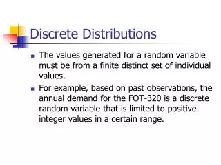
Random Variables of the Discrete Type • When S contains a countable number of points, • X can be defined to correspond each point in S to a positive integer. • S is a set of discrete points or a discrete outcome space. • X is a random variable of discrete type. • The probability mass function (p.m.f.) f(x) denotes P(X=x). • f(x) is also called probability function, probability density function, frequency function. • Def.3.1-2: f(x) of a discrete random variable X is a function: • f(x)>0, x ∈S. • ∑x∈Sf(x) = 1, • P(X∈A) = ∑x∈Af(x), where A ⊂S. • f(x)=0 if x ∉S: S is referred to as the supportof X and the space of X. • A distribution is uniformif its p.m.f. is constant over the space. • For instance, f(x)=1/6 in rolling a fair 6-sided dice. • Ex.3.1-3: Roll a 4-sided die twice and let X be the largest of two outcomes. S={(i, j): i, j=1..4}. P(X=1)=P({(1,1)})=1/16. P(X=2)=P({(1,2), (2,1), (2,2)})=3/16, …, f(x)=P(X=x)=(2x-1)/16 for x=1..4; f(x)=0 otherwise.
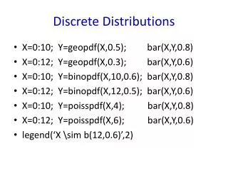
Graphing the Distribution • (a) For a discrete probability distribution, we simply plot the points (x, f(x)) , for all x R . • (b) To get a better picture of the distribution, we use bar graphs and histograms . • (c) A bar graph is simply a set of lines connecting (x, 0) and (x, f(x)) . • (d) If X takes on only integer values, then a histogram can be used by using rectangles centered at each x R of height f(x) and width one.
Graphic Representation of f(x) • The graph consists of the set of points {(x, f(x): x∈S}. • Better visual appreciation: a bar graph, a probability histogram. • P(X=x)=f(x)=(2x-1)/16, x=1..4. • Hyper-geometric distribution: a collection has N1 objects of type 1 and N2 objects of type 2. X is the number of type-1 objects in the n objects taken from the collection w/o replacement.
Examples • Ex.3.1-5: In a pond of 50 fish with 10 tagged, 7 fish are caught at random w/o replacement. • The probability of 2 tagged fish caught is • Ex.3.1-7: In a lot of 25 items with unknown defective, 5 items are selected at random w/o replacement for exam. • If no defective found, the lot is accepted; otherwise, rejected. • Given N1 defective, the acceptance probability, operating characteristic curve, is • Ex.3.1-8: Roll a 4-sided die twice. X is the sum: 2..8. • f(x)=(4-|x-5|)/16. • 1000 experiments simulated on a computer.
Mathematical Expectation • Def.3.2-1: For a random variable X with p.m.f. f(x), if ∑x∈Su(x)f(x) exists, it is called the mathematical expectationor the expected valueof the function u(X), denoted by E[u(X)]. • It is the weighted mean of u(x), x∈S. • The function u(X) is also a random variable, say Y, with p.m.f. g(y). • Ex.3.2-2: For a random variable X with f(x)=1/3, x∈S={-1, 0, 1}. • Let u(X)=X2. Then, E[u(X)]= E[X2]=2/3. • The support of the random variable Y=X2 is S1={0, 1}, and P(Y=0)=P(X=0), P(Y=1)=P(X=-1)+P(X=1), so its p.m.f. • Hence ∑y∈S1yg(y) = 2/3, too. • Thm.3.2-1: mathematical expectation E, if exists, satisfies: • For a constant c, E(c)=c. • For a constant c & a function u, E[c u(X)]=c E[u(X)]. • For constants a & b and functions u & v, E[a u(X) + b v(X)]=a E[u(X)] + b E[v(X)]. • It can be applied for 2+terms since E is a linearor distributiveoperator.
Examples • Ex3.2-3: f(x)=x/10, x=1,2,3,4. • Ex3.2-4: u(x)=(x-b)2, where b is a constant. • Suppose E[(X-b)2] exists. What is the value of b to minimize it? • Ex3.2-5: X has a hypergeometric distribution.
More Examples • Ex.3.2-6: f(x)=x/6, x=1,2,3. • E(X)=μ=1(1/6)+2(1/6)+3(1/6)=7/3. • Var(X)=σ2=E[(X-μ)2]=E(X2)-μ2=…=5/9 ⇒ σ=0.745 • Ex.3.2-7: f(x)=1/3, x=-1,0,1. • E(X)=μ=-1(1/3)+0(1/3)+1(1/3)=0. • Var(X)=σ2=E(X2)-μ2=…=2/3⇒The standard deviation σ=0.816 • Comparatively, g(y)=1/3, y=-2,0,2. • Its mean is also zero; but, Var(Y)=8/3 and σY=2σ. ⇒ more spread out. • Ex.3.2-8: uniform f(x)=1/m, x=1..m. • E(X)=μ=1(1/m)+…+m(1/m)=(m+1)/2. • Var(X)=σ2=E(X2)-μ2=…=(m2-1)/12 • For instance, m=6 when rolling a 6-sided die.
Derived Random Variables • Linear Combination: X has a mean μX and variance σX2. • Y=aX+b⇒μY = aμX+b; Var(Y)=E[(Y-μY)2] =…=a2σX2; σX=|a|σX. • a=2, b=0 ⇒mean*2, variance*4, standard deviation*2. • a=1, b=-1 ⇒mean-1, variance*1, standard deviation*1. Var(X-1) = Var(X). • The rthmoment of the distribution about b: E[(X-b)r]. • The rth factorial moment: E[(X)r]=E[X(X-1)(X-2)…(X-r+1)]. • E[(X)2] = E[X(X-1)] = E(X2)-E(X) = E(X2)-μ. • E[(X)2]+μ-μ2= E(X2)-μ+μ-μ2= E(X2)-μ2= Var(X)=σ2. • Ex3.2-9: X has a hypergeometric distribution. (ref. Ex3.2-5)
Bernoulli Trials • A Bernoulli experimentis a random experiment, whose outcome can be classified in one of two mutually exclusive and exhaustive ways: success or failure. • A series of Bernoulli trialsoccurs after independent experiments. • Probabilities of success p and failure q remain the same. (p+q=1) • Random variable X follows a Bernoulli distribution. • X(success)=1 and X(failure)=0. • The p.m.f. of X is f(x)=pxq(1-x), x=0,1. • (μ, σ2)=(p, pq). • A series of n Bernoulli trials, a random sample, will be an n-tuple of 0/1’s. • Ex.3.3-4: Plant 5 seeds and observe the outcome (1,0,1,0,1): 1st, 3rd, 5th seeds germinated. If the germination probability is .8, the probability of this outcome is (.8)(.2)(.8)(.2)(.8) assuming independence. • Let X be the number of successes in n trials. • X follows a binomial distribution, denoted as b(n, p). • The p.m.f. of X is
Example • Ex.3.3-5: For lottery with .2 winning, if X equals the number of winning tickets among n=8 purchases. • The probability of having 2 winning tickets is • Ex.3.3-6: The effect of n and p is illustrated as follows.
Cumulative Distribution Function • The cumulative probability F(x), defined as P(X≤ x), is called the cumulative distribution functionor the distribution function. • Ex.3.3-7: Assume the distribution of X is b(10, 0.8). • F(8) = P(X≤8) = 1-P(X=9)-P(X=10) = 1-10(.8)9(.2)-(.8)10=.6242. • F(6) = P(X≤6) = ∑x=0..6Cx10 (.8)x(.2)10-x. • Ex.3.3-9: Y follows b(8, 0.65). • If X=8-Y, X has b(8, .35), whose distribution function is in Table II (p.647). • E.g., P(Y≥6) = P(8-Y≤8-6) = P(X≤2)=0.4278 from table lookup. • Likewise, P(Y≤5) = P(8-Y≥8-5) = P(X≥3) = 1-P(X≤2) = 1-0.4278 =0 .5722. • P(Y=5) = P(X=3) = P(X≤3)-P(X≤2) = 0.7064-0.4278 = 0.2786. • The mean and variance of the binomial distribution is (μ, σ2)=(np, npq). • Ex.3.4-2 details the computations.
Comparisons • Empirical Data vs. Analytical Formula: • Ex.3.3-11: b(5, .5) has μ= np= 2.5, σ2= npq= 1.25. • Simulate the model for 100 times: 2, 3, 2, …⇒ = 2.47, s2=1.5243. • Suppose an urn has N1success balls and N2 failure balls. N = N1+ N2. • Let p = N1/N, and X be the number of success balls in a random sample of size n taken from this urn. • If the sampling is done one at a time with replacement, X follows b(n, p). • If the sampling is done without replacement, X has a hypergeometric distribution with p.m.f. • If N is large and n is relative small, it makes little difference if the sampling is done with or without replacement. (See Fig.3.3-4)
Moment-Generating Function (m.g.f ) • Def.3.4-1: X is a random variable of the discrete type with p.m.f. f(x) and space S. If there is a positive integer h s.t. • E(etX) = ∑x∈Setxf(x) exists and is finite for –h<t<h, then M(t) = E(etX) is called the moment-generating functionof X. • –E(etX) exists and is finite for –h<t<h ⇔M(r)(t) exist at t=0, r=1,2,3,… • –Unique association: p.m.f. ⇔m.g.f. • Sharing the same m.g.f., two random variables have the same distribution of probability. • Ex.3.4-1: X has m.g.f M(t) = et(3/6)+ e2t(2/6)+ e3t(1/6). • From e“x”t, Its p.m.f. has f(0)=0, f(1)=3/6, f(2)=2/6, f(3)=1/6, f(4)=0, … • Therefore f(x)=(4-x)/6, x=1,2,3.. • Ex.3.4-2: X has m.g.f M(t) = et/2(1-et/2), t<ln2. • (1-z)-1= 1 + z + z2+ z3+ …, |z|<1.
Application of Application of m.g.f • M(t) = E(etX) = ∑x∈Setxf(x) exists and is finite for –h<t<h. M'(t) = ∑x∈Sxetxf(x), M'(0) = ∑x∈Sxf(x) = E(X), M''(t) = ∑x∈Sx2etxf(x), …, M''(0) = ∑x∈Sx2f(x) = E(X2), …, M(r)(t) = ∑x∈Sxretxf(x). M(r)(0) = ∑x∈Sxrf(x) = E(Xr), as t=0. • M(t) must be formulated (in closed form) to get its derivatives of higher order. • Ex.3.4-3: X has a binomial distribution b(n, p). • Thus, its m.g.f. is • When n=1, X has a Bernoulli distribution.
Negative Binomial Distribution • Let X be the number of Bernoulli trials to observe the rth success. • X has a negative binomial distribution. • Its p.m.f. g(x) is • If r=1, X has a geometric distributionwith
Geometric Distribution • X has a geometric distribution with the p.m.f. • P(X > k), P(X ≤k): • Memory-less: • (EX3.412) • Ex3.4-4: Fruit flies’ eyes with ¼white and ¾red. • The probability of checking at least 4 flies to observe a white eye is P(X≥4) = P(X>3) = (¾)3= 0.4219. • The probability of checking at most 4 flies to observe a white eye isP(X≤4) = 1-(¾)3=0.6836. • The probability of finding the first white eye on the 4th fly checked is P(X=4) = pq4-1= 0.1055. <= P(X≤4) -P(X≤3) • Ex3.4-4: For a basketball player with 80% free throw. • X is the minimum number of throws for a total of 10 free throws. • Its p.m.f. is • μ= r/p= 10/0.8 = 12.5, σ2= rq/p2= 10(0.2)/(0.8)2= 3.125.
m.g.f. . ⇒ p.d.f • By Maclaurin’sseries expansion (ref. p.632): If the moments of X, E(Xr) = M(r)(0), are known, M(t) is thus determined. ⇒ p.d.f. can be obtained by rewriting M(t) as the weighted sum of e“x”t. • Ex3.4-7: If the moments of X are E(Xr) = 0.8, r=1,2,3,… • Then, M(t) can be determined as Therefore, P(X=0)=0.2 and P(X=1)=0.8
Poisson Process • Def.3.5-1: An approximate Poisson process with parameter λ>0: • The numbers of changes occurring in non-overlapping intervals are independent. • The probability of exactly one change in a sufficiently short interval of length h is approximately λh. • The probability of two or more changes in a sufficiently short interval is essentially zero. • Determine p.m.f.: • During the unit interval of length 1, there are x changes. • For n»x, we partition the unit interval into n subintervals of length 1/n. • The probability of x changes in the unit interval ≡The probability of one change in each of exactly x of these n subintervals. • The probability of one change in each subinterval is roughly λ(1/n). • The probability of two or more changes in each subinterval is essentially 0. • The change occurrence or not in each subinterval becomes a Bernoulli trial. • Thus, for a sequence of n Bernoulli trials with probability p = λ/n, P(X=x) can be approximated by (binomial):
Examples • Ex.3.5-1: X has a Poisson distribution with a mean of λ=5. • Table III on p. 652 lists selected values of the distribution. • P(X≤6) = 0.762 • P(X>5) = 1-P(X≤5) = 1-0.616 =0.384 • P(X=6) = P(X≤6)-P(X≤5) = 0.762-0.616 = 0.146 • Ex.3.5-2: The Poisson probability histograms:
More Examples • Empirical data vs. Theoretical formula (Ex.3.5-3) • X is the number of αparticles emitted by barium-133 in .1 sec and counted by a Geiger counter. • 100 observations are made. • Generally with unit interval of length t, the Poisson p.m.f. is • Ex.3.5-4: Assume a tape flaw is a Poisson distribution with a mean of λ= 1/1200 flaw per feet. • What is the distribution of X, the number of flaws in a 4800-foot roll? • E(X)=4800/1200=4. • P(X=0) = e-4= 0.018 • By Table III on p. 652, P(X≤4) =0 .629
When Poisson ≈ Binomial • Poisson with λ=np can simulate Binomial for large n and small p. • (μ, σ2)=(λ, λ) ≈(np, npq). • Ex3.5-6: Bulbs with 2% defective rate. • The probability that a box of 100 bulbs contains at most 3 defective bulbs is • By Binomial, the tedious computation will result in • Ex3.5-7: p.160, the comparisons of Binomial and Poisson distributions.
When Poisson ≈ Binomial Binomial ≈ Hypergeometric Hypergeometric • Ex3.5-8: Among a lot of 1000 parts, n=100 parts are taken at random w/o replacement. The lot is accepted if no more than 2 of100 parts taken are defective. Assume p is the defective rate. • Operating characteristic curve OC(p) = P(X≤2) = P(X=0)+P(X=1)+P(X=2). Hypergeometric:N1=1000p,N=1000, N2=N-N1 • Since N is large, it makes little difference if sampling is done with or without replacement. ⇒simulated by Binomial! • n Bernoulli trials: • For small p, p=0~.1: ⇒simulated by Poisson! • OC(0.01)=0.92OC(0.02)=0.677OC(0.03)=0.423OC(0.05)=0.125OC(0.10)=0.003