Download

1 / 30
310 likes | 537 Views
Informed Search and Exploration. Search Strategies Heuristic Functions Local Search Algorithms. Vilalta&Eick: Informed Search. Introduction. Informed search strategies: Use problem specific knowledge Can find solutions more efficiently than

E N D
Informed Search and Exploration • Search Strategies • Heuristic Functions • Local Search Algorithms Vilalta&Eick: Informed Search
Introduction • Informed search strategies: • Use problem specific knowledge • Can find solutions more efficiently than search strategies that do not use domain specific knowledge.
Greedy Best-First Search • Expand node with lowest evaluation function f(n) • Function f(n) estimates the distance to the goal. Simplest case: f(n) = h(n) estimates cost of cheapest path from node n to the goal. ** HEURISTIC FUNCTION **
Greedy Best-First Search • Resembles depth-first search • Follows the most promising path • Non-optimal • Incomplete
A* Search Evaluation Function: F(n) = g(n) + h(n) Estimated cost of cheapest path from node n to goal Path cost from root to node n
A* Search; optimal Optimal. • Optimal if admissible heuristic • admissible: Never overestimates the cost • to reach a goal from a given state.
A* Search; optimal • Assume optimal solution cost is C* • Suboptimal node G2 appears on the fringe: f(G2) = g(G2) + h(G2) > C* • Assume node n is an optimal path: f(n) = g(n) + h(n) <= C* Therefore f(n) < C* < f(G2)
A* Search; complete • A* is complete. • A* builds search “bands” of increasing f(n) • At all points f(n) < C* • Eventually we reach the “goal contour” • Optimally efficient • Most times exponential growth occurs
Contours of equal f-cost 400 420
Data Structures of Expansion Search • Search Graph:= discussed earlier • Open-list:= set of states to be expanded • Close-list:= set of states that have already been expanded; many implementation do not use close-list (e.g. the version of expansion search in our textbook) potential overhead through looping but saves a lot of storage
Problem: Expansion Search Algorithms Frequently Run Out of Space Possible Solutions: • Restrict the search space; e.g. introduce a depth bound • Limit the number of states in the open list • Local Beam Search • Use a maximal number of elements for the open-list and discard states whose f-value is the highest. • SMA* and MA* combine the previous idea and other ideas • RBFS (mimics depth-first search, but backtracks if the current path is not promising and a better path exist; advantage: limited size of open list, disadvantage: excessive node regeneration) • IDA* (iterative deepening, cutoff value is the smallest f-cost of any node that is greater than the cutoff of the previous iteration)
Local beam search • Keep track of best k states • Generate all successors of these k states • If goal is reached stop. • If not, select the best k successors • and repeat.
Learning to Search The idea is to search at the meta-level space. Each state here is a search tree. The goal is to learn from different search strategies to avoid exploring useless parts of the tree.
Informed Search and Exploration • Search Strategies • Heuristic Functions • Local Search Algorithms
8-Puzzle Common candidates: F1: Number of misplaced tiles F2: Manhattan distance from each tile to its goal position.
How to Obtain Heuristics? • Ask the domain expert (if there is one) • Solve example problems and generalize your experience on which operators are helpful in which situation (particularly important for state space search) • Try to develop sophisticated evaluation functions that measure the closeness of a state to a goal state (particularly important for state space search) • Run your search algorithm with different parameter settings trying to determine which parameter settings of the chosen search algorithm are “good” to solve a particular class of problems. • Write a program that selects “good parameter” settings based on problem characteristics (frequently very difficult) relying on machine learning
Informed Search and Exploration • Search Strategies • Heuristic Functions • Local Search Algorithms
Local Search Algorithms • If the path does not matter we can deal with local search. • They use a single current state • Move only to neighbors of that state • Advantages: • Use very little memory • Often find reasonable solutions
Local Search Algorithms • It helps to see a state space landscape • Find global maximum or minimum Complete search: Always finds a goal Optimal search: Finds global maximum or minimum.
Hill Climbing • Moves in the direction of increasing value. • Terminates when it reaches a “peak”. • Does not look beyond immediate neighbors (variant: use definition of a neighborhood later).
Hill Climbing Can get stuck for some reasons: • Local maxima • Ridges • Plateau Variants: stochastic hill climbingmore details later • random uphill move • generate successors randomly until one is better • run hill climbing multiple times using different initial states (random restart)
Simulated Annealing • Instead of picking the best move pick • randomly • If improvement is observed, take the step • Otherwise accept the move with some • probability • Probability decreases with “badness” of step • And also decreases as the temperature goes • down
Example of a Schedule Simulated Annealling T=f(t)= (2000-t)/2000 --- runs for 2000 iterations Assume E=-1; then we obtain t=0 downward move will be accepted with probability e-1 t=1000 downward move will be accepted with probability e-2 t=1500 downward move will be accepted with probability e-4 t=1999 downward move will be accepted with probability e-2000 Remark: if E=-2 downward moves are less likely to be accepted than when E=-1 (e.g. for t=1000 a downward move would be accepted with probability e-4)