Download

1 / 34
340 likes | 447 Views
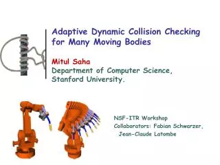
This research paper explores methods for efficient collision checking in scenarios with many moving bodies and provides a generalized bisection method for such scenarios. It introduces the concept of adaptive resolution collision checking to ensure exact collision detection. The study covers various techniques and heuristics to improve collision checking speed and accuracy.

E N D
Adaptive Dynamic Collision Checking for Many Moving BodiesMitul SahaDepartment of Computer Science,Stanford University. NSF-ITR Workshop Collaborators: Fabian Schwarzer, Jean-Claude Latombe
Static vs. Dynamic Collision Checking Static Dynamic • Static collision checking tests a single configuration q for collision • Dynamic collision checking ensure that all configurations on a continuous path are collision-free.
Motivation (1) Bottleneck in PRM planning: Efficient testing of sampled configurations and connections for collision. qb qa (Usually people trade-off reliability for speed in dynamic collision checking.)
[Quinlan, 94] [Gottschalk, Lin, Manocha, 96] Motivation (2) Static collision tests (for sampled configurations) are done efficiently using pre-computed bounding volume (BV) hierarchies A B
Motivation (3) Butdynamic collision tests (for connections betweensampled configurations) using BV hierarchies are usually approximate. 3 2 3 1 3 2 3 • too large collisions are missed • too small slow test of local paths
Motivation (3) Butdynamic collision tests (for connections betweensampled configurations) using BV hierarchies are usually approximate.
Previous Approaches to Dynamic Collision Testing • Bounding-volume (BV) hierarchies Discretization issue • Feature-tracking methods[Lin, Canny, 91] [Mirtich, 98] V-Clip [Cohen, Lin, Manocha, Ponamgi, 95] I-Collide [Basch, Guibas, Hershberger, 97] KDS Geometric complexity issue with highly non-convex objects Sequential strategy (first collision) that is not efficient for PRM path segments • Swept-volume intersection[Cameron, 85] [Foisy, Hayward, 93] Swept-volumes are expensive to compute. Too much data. No pre-computed BV hierarchies • Algebraic trajectory parameterization[Canny, 86] [Schweikard, 91] [Redon, Kheddar, Coquillard, 00] High-degree polynomials, expensive • Combination[Redon, Kheddar, Coquillard, 00] BVH + algebraic parameterization [Ehmann, Lin, 01] BVH + feature tracking Sequential strategy
Desirables in Nutshell • Adaptive resolution • Exact collision checking • Competitive with discrete checkers w.r.t. speed
Definitions Workspace C-space Ai (qb) qb i (qa,qb) qb qa qa Ai (qa) • i(qa,qb)≡curveLength(Ai) on qa…qb
Definitions Workspace C-space Ai (qb) Aj (qb) • ij(q)≡distance(Ai, Aj) • ij(q)= 0 Collision qb ηij (qb) qb qa qa
Key Lemma: If i (qa,qb) + j (qa,qb) < ηij (qa) + ηij (qb), then there exists no collision between Ai and Aj along qa-qb Key Lemma Workspace C-space Ai (qb) Aj (qb) qb ηij (qb) i (qa,qb) j (qa,qb) qb qa ηij (qa) qa Aj (qa) Ai (qa)
Key Lemma: If i (qa,qb) + j (qa,qb) < ηij (qa) + ηij (qb), then there exists no collision between Ai and Aj along qa-qb • Intuition behind the key lemma: Key Lemma Aj i Ai ηij i < ηijSafe
i (qa,qb) + j (qa,qb) < ηij (qa) + ηij (qb) Collision -free If i (qa,qb) + j (qa,qb) ηij (qb) ηij (qa) else Not sure! Hence bisect Collision Checking using the Lemma
Collision Checking using the Lemma • After the collision check a collision-free connection may look like: • Each sub-segment segment satisfies the lemma: i (qa,qb) + j (qa,qb) < ηij (qa) + ηij (qb) and hence the collision checking is exact • The collision checking is adaptive
Generalization:Large Number of Moving Bodies • Robot(s) and static obstacles treated as collection of rigid bodies A1, …, An. • If i(q,q’) + j(q,q’) < ij(q) + ij(q’)then Ai and Aj do not collide between q and q’
Generalized Bisection Method for Large Number of Moving Objects • Each pair of bodies is checked independently of the others priority queue Q of elements [qa,qb]ij • Initially, Q consists of [q,q’]ij for all pairs of bodies Ai and Aj that need to be tested. • Until Q is not empty do: • [qa,qb]ij remove-first(Q) • If i(qa,qb) + j(qa,qb) ij(qa) + ij(qb) then • qmid (qa+qb)/2 • If ij(qmid) = 0 then return collision • Else insert [qa,qmid]ij and [qmid,qb]ij into Q • Return no collision
Heuristic Ordering Q • Goal:Discover collision quicker if there is one. • Sort Q by decreasing values of:[li(qa,qb) + lj(qa,qb)] – [hij(qa) + hij(qb)]
Generalized Bisection Method for Large Number of Moving Bodies • Things to note: • Different pair of bodies tested with different resolutions, i.e. usually close pair of objects are checked with finer resolution than the distant ones. • Usually close pair of objects are considered before the distant ones.
i (qa,qb) + j (qa,qb) < ηij (qa) + ηij (qb) How do we getij(q)andi(qa,qb)? ij(q) Aj(q) Calculating Terms in the Key Lemma i(qa,qb) Ai(q) Ai(qa) Aj(qb)
Lower bound on Distance between Bodies • Need to find ηij’s • Exact and approximate distance computations are very expensive compared to pure collision checking • So is there any alternative? Aj Aj ηij
Lower bound on Distance between Bodies • Use a classical BVH collision checker with a slight modification • Compute distance between BVs instead of just testing BV overlap BVs are RSSs ij(q) • returns values often much larger than ½ distances • much faster than BV-based exact or ½-approximate distance computation • almost as fast as pure collision checking
i (qa,qb) + j (qa,qb) < ηij (qa) + ηij (qb) How do we getij(q)andi(qa,qb)? ij(q) Aj(q) Calculating Terms in the Key Lemma i(qa,qb) Ai(q) Ai(qa) Aj(qb)
A4 q4 ( q , q ) L q q 1 a b a , 1 b , 1 A3 ( q , q ) 2 L q q L q q 2 a b a , 1 b , 1 a , 2 b , 2 q3 q2 ( q , q ) ( 2 L D ) q q 3 a b a , 1 b , 1 A2 ( L D ) q q q q a , 2 b , 2 a , 3 b , 3 A1 ( q , q ) ( 3 L D ) q q q1 4 a b a , 1 b , 1 ( 2 L D ) q q q q a , 2 b , 2 a , 3 b , 3 L q q a , 4 b , 4 Bounding Motions in Workspace i(qa,qb) Rigid Body Upper Bound Path Length A1 A2 A3 A4
Comparative Experiment • SBL: PRM planner (single-query, bi-directional, lazy in cc) with fixed-discretization collision checker • A-SBL: Same planner, with new collision checkerExperiment: • Run SBL 10 times on same planning problem with some resolution e • If a collision has been missed, reduce e and repeat • If no collision has been missed, return average planning time • Run A-SBL 10 times and return average planning time Robot: 2,502 triangles Obstacles: 432 Triangles SBL 17 sec A-SBL 4.8 sec
Some Result Robot: 2,502 triangles Obstacles: 432 Triangles SBL 17 sec A-SBL 4.8 sec Robot: 2,991 triangles Obstacles: 432 Triangles SBL 83 sec A-SBL 44 sec Robot: 2,991 trianglesObstacles: 74,681 triangles SBL 1.20 sec A-SBL 0.81 sec Robot: 2,502 trianglesObstacles: 34,171 triangles SBL 3.2 sec A-SBL 2.1 sec Robots: 6 x 2,991 trianglesObstacles: 19,668 triangles SBL 85 sec A-SBL 52 sec
Summing up.. • New dynamic collision checker which: • Never misses a collision • Eliminates need for determining resolution factor: e • Is even faster than the discrete checker in PRM planning • Techniques that considerably improve efficiency: • Greedy Distance Computation algorithm, nearly as efficient as pure collision checker • Fast technique for bounding lengths of paths traced out in workspace • Heuristics for ordering collisions tests • Represent deformable objects with a large number of small rigid objects vs
Summing up.. • A free downloadable c++ implementation of the new dynamic collision checker is on the web: http://robotics.stanford.edu/~mitul/mpk
NSF-ITR Workshop Collaborators: Fabian Schwarzer, Jean-Claude Latombe Adaptive Dynamic Collision Checking for Many Moving ObjectsMitul SahaDepartment of Computer ScienceStanford University Any Question?
SBL X [Sanchez-Ante, Latombe, 01]
mg mb SBL [Sanchez-Ante, Latombe, 01]
Our New Collision Checker • Based on “Adaptive Bisection” • Ideas: • Relate configuration changes to path lengths in workspace • Use distance computation rather than pure collision checking
Current Research • Extension to deformable objects • Large number of small bodies can be used to approximate • deformable objects