Download
1 / 31
310 likes | 566 Views
Business Cycles, Macro Variables, and Stock Market Returns. William Carter, David Nawrocki, and Tonis Vaga. Agenda. Introduction and literature review (Jon) Relationships between real activity and stock returns (Jordan) Multiple phases of the business cycle (Danielle)

E N D
Business Cycles, Macro Variables, and Stock Market Returns William Carter, David Nawrocki, and Tonis Vaga
Agenda • Introduction and literature review (Jon) • Relationships between real activity and stock returns (Jordan) • Multiple phases of the business cycle (Danielle) • Linear regression analysis (Dmitry) • Application of neural network (Raegen) • Conclusion (Jon)
Introduction • Business cycle indicators: relevant issue • Chen, Roll, and Ross; Fama and French; and Schwert • Risk premium embedded in expected returns moves inversely with business conditions • Whitelaw • Conditional returns and conditional volatility change over time with changes in the cycle • Nawrocki and Chauvet • Find dynamic relationship between stock market fluctuations and cycles
Intro. Con’t. • Perez-Quiros and Timmerman • Asymmetries in conditional mean and volatility of excess stock returns around cycle turning points • Chauvet and Porter • Suggest non-linear risk measure that allows risk-return relationship to not be constant over Markov states • DeStafano • Tests four-state model of cycle and dividend discount model to provide evidence that expected stock returns vary inversely with economic conditions
This all suggests… • Nonlinear financial market dynamic • Thus requiring a nonlinear methodology • Between business cycle and stock market • DeStafano (2004) • Arbitrarily defined four phases • Period between NBER peaks and troughs into two equal periods
Where the authors differ • Utilizes simple linear models • Looks for phase transitions • Provides preliminary definitions of phases • Then used in the neural network methodology for final estimates of the phases • Independent of NBER peaks and troughs • Not announced until 9-18 months after the fact
Multiple Phases of the Business Cycle • Chauvet and Potter (1998) and Perez-Quiros and Timmermann (2000) study two phases: expansions and recessions • Consistent with the NBER’s definition of business cycle peaks and troughs • Chauvet and Potter (1998) note changes in conditional means and variances well before the peak and trough, suggesting additional phases of the business cycle • Four/five-stage models have been proposed by Hunt (1987), Stovall (1996), DeStefano (2004), Guidolin and Timmermann (2005), Guidolin and Ono (2006)
Advantages of the Neural Network • Eliminates problems from traditional approaches • Linearity assumptions • Data-pooling issues • Data mining • Pre-specification of the model
Relationships between Real Activity and Stock Returns • Prior Research: • Moore (1976) and Sherman (1986) found certain economic indicators are leading indicators for the business cycle and security markets • Chen, Roll, Ross (1986) modeled equity returns using macroeconomic factors: • Industrial Production • Monetary Aggregates • Debt Market Yields • Fama & French (1989) measured stock return volatility using the relationship between returns and real activity
Skewness • Skewness and volatility has also been tied to the business cycle • Schwert (1989) finds stock market volatility increases during recessions • Other research has found high variability in the skewness of stock returns and that it varies systematically with business conditions • Skewness becomes more negative during expansions and less negative or positive during contractions
Prior Research • Whitelaw (1994) finds that the relationship between the conditional mean and volatility of stock returns is nonstationary • Using a linear relationship between mean and volatility can lead to incorrect results from GARCH and ARCH models • Utilizing a Nonlinear Markov switching regression: • Volatility increases during recessions • Conditional means rise before the end of recessions • Conditional means decrease before the peak of expansions • Sharpe ratios are negative in troughs, positive in peaks
Prior Research • Whitelaw (1994) et al. find conditional variance is countercyclical • Fama and French (1989) et al. find conditional means move with the business cycle • Rapach (2001) finds real stock returns are related to changes in money supply, aggregate supply, aggregate spending • This research suggests that stock market phases are related to economic fluctuations
Prior Research • Recent research finds that the power of the economic factors used for predictions varies over time and volatility • Small firms are shown to be strongly affected during recessions • Fundamental factors such as DDM are affected by the business cycle • Investors discount earnings using short term T-Bill when the economy is slowing down • Discount using long term T-Bond rate in the other states of economy
Method • Time-invariant forecasting models will not work under sudden large changes in time series • Previous research was determined using the NBER cycle dates, which have a lag of 9 – 18 months • The Markov switching VAR is used in this study along with a neural network • It does not require the form of the regression to be previously specified • Allows for a state switching nonlinear model that tests the significance of the various macroeconomic variables • The neural network must be provided with an initial set of dates for the phases and macroeconomic variables for the transistions
Multiple Phases of the Business Cycle • Chauvet and Potter (1998) and Perez-Quiros and Timmermann (2000) study two phases: expansions and recessions • Consistent with the NBER’s definition of business cycle peaks and troughs • Chauvet and Potter (1998) note changes in conditional means and variances well before the peak and trough, suggesting additional phases of the business cycle • Four/five-stage models have been proposed by Hunt (1987), Stovall (1996), DeStefano (2004), Guidolin and Timmermann (2005), Guidolin and Ono (2006)
Stovall’s Business Cycle Phases • Expansion in 3 phases: • Recovery from recession – slow growth • Economic growth picks up vigorously • Inflation increases • Recession in 2 phases: • Decline in economic production • Economy flattens out and begins to recover • A simplistic model – Stovall uses the time period between NBER peaks and troughs, divides each time period evenly into three and two periods • Finds that certain sectors perform well during certain stages
Hunt’s Business Cycle Phases • Hunt suggests economic variables that drive the transition between phases • Easeoff • Industrial production slows • Initial unemployment claims increase • Non-farm payrolls turn down • University of Michigan Consumer Sentiment index falls • Plunge • Federal Funds rate decreases • Real monetary base increases • Interest rate spread narrows • Revival • Industrial production increases • Initial unemployment claims fall • Non-farm payrolls increase • Acceleration • Real monetary base increases • Consumer Price Index rises • Early Revival – transition between Plunge and Revival
Hunt’s Business Cycle Phases • Implemented his model using 12-month rate of change statistics, followed monthly • One complete cycle measured from Easeoff to Easeoff phase • Each phase exhibited different investment behavior • Easeoff had significant negative skewness • Consistent with Alles and Kling’s (1994) finding that skewness becomes strongly negative during contractions • Plunge had insignificant skewness • Revival had initial insignificant skewness, followed by positive significant skewness • Acceleration exhibited poor risk-return behavior (high inflation period) • Easeoff and revival exhibited the best risk-return behavior
Linear regression analyses • Two regression analyses performed on monthly time series for the period 1970-1997 to study relationships between S&P 500 and variables • Macroeconomic variables considered • CPI rate of change (CPIROC) • Industrial production rate of change (IP) • Spread between 90-days T-bill and 30-year T note (SPREAD) • Difference between AAA and BAA corporate bonds (AAA_BAA) • Rate of change in real adjusted monetary base lagged 4 month (REAL_MB) • Level of housing starts (STARTS) • Level of manufacturing orders excluding aircraft and parts (ORDERS)
Regression results for 1971-1997 • Industrial production, manufacturing orders, and housing starts are significant at 10% confidence level • The correlation between independent variables is quite low below 0.40. Only two correlation coefficients were as high as 0.60 • Adjusted R2 below 0.0386 indicates little relationship between variables
Individual regression results for four business cycle phases
Individual regression results for four business cycle phases (cont.) • Impact of variables changes through the phases of the business cycle • All of the phase regressions have higher adjusted R2 compared to the base regression • The four phase regressions exhibit different significant independent variables both from each other and the base regression • Conclusion: strong support for the hypothesis that S&P 500 has different phases
Studying Economic Phases with a Neural Network • What is a neural network? • Mimics the structure of the brain. Output is produced by interconnected nodes in a parallel fashion as opposed to traditional sequential processing. • This operation makes the NN more robust and adaptable to fuzzy logic. • Here, a neural network is used as computational architecture to learn from past economic phases and performance variables. And, then predict unseen phases in the economy.
Studying Economic Phases with a Neural Network • Advantages of using a Neural Network • Captures all relationships (linear and non) • A pre-specified regression equation is not required • This study uses a PNN • PNN’s use estimated “probability functions to train the network with a data set.” • It is an adaptive PNN, meaning that an algorithm determines a smoothing function for each variable. The variables can be weighted and insignificant variables eliminated.
Studying Economic Phases with a Neural Network • How it works • The neural network was trained, using 1971 to 1988, to specify the phase for the next year. • After each 12 month period was added on the network retrained • Testing the neural network • Known economic phases for Dec 1989 through Dec 1997 were compared to the neural network’s defined phases • Linear and nonlinear models differ 37% of the time…indicating that there is some nonlinear dynamic captured by the NN. • “There are significant variables and processes in the S&P data stream that are not strictly linear. Linear models can only approximate the actual nonlinear process.”
Studying Economic Phases with a Neural Network …Since 1997
Summary and Conclusions • Previous research • Two market states in economy and US stock market returns (S&P 500 index) • Four, possibly five Markov states have been identified in the business cycle • Regression analysis and neural network provide evidence of four distinct market states • Supports empirical research that delineates 4-5 market states
Summary and Conclusion Con’t. • Instead of a fundamental variable approach using earnings and discount rates (DeStafano) • Macroeconomic variable approach was used • Real time approach • Even though independent of NBER • NBER peak occurs in Easeoff/Plunge phases • NBER trough occurs in Plunge/Revival phases
Summary and Conclusion Con’t. • This methodology closely corresponds to the “growth cycle” methodology defined by Geoffrey H. Moore • Also supports studies that discovered nonlinear relationships in financial markets • Chauvet and Potter (1998) • Perez-Quiros and Timmermann (2000) • Echo LeBaron’s warning • Results with nonlinear measures are not as robust as results obtained from linear models
Step Back….. • These different business cycles could be used for the Coleman Fund • To switch out of potentially underperforming sectors • QInsight has the economy in the plunge phase • In general, if these criteria were used we would be invested in a slightly different combination of sectors