Download
1 / 42
420 likes | 594 Views
Seminar in Phylogeny, CS236805. Linear Least Squares and its applications in distance matrix methods. Presented by Shai Berkovich June, 2007. Based on the paper by Olivier Gascuel. Contents. Background and Motivation LS in general LS in phylogeny UNJ algorithm LS sense of UNJ.

E N D
Seminar in Phylogeny, CS236805 Linear Least Squares and its applications in distance matrix methods Presented by Shai Berkovich June, 2007 Based on the paper by Olivier Gascuel
Contents • Background and Motivation • LS in general • LS in phylogeny • UNJ algorithm • LS sense of UNJ
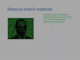
Distance Matrix Methods A major family of phylogenic methods has been the distance matrix methods. The general idea: calculate a measure of the distance between each pair of species, and then find a tree that predicts the observed set of distances as closely as possible.
Distance Matrix Methods This lives out all information from higher-order combinations of character states, reducing the data matrix to a simple table of pairwise distances, though computer simulation studies show that the amount of information of phylogeny that is lost is remarkably small. (As we already saw: Neighbor-Joining and its robustness to noise.)
Additivity Definition: A distance matrix D is additive if there exists a tree with positive edge weights such that where vk are the edges in the path between species i and j. Theorem [Waterman et. al., 1977]: Given ad additive n x n distance matrix D there is a unique edge-weighted tree (without nodes of degree 2) in which n nodes in the tree are labeled s1,s2,…,snso that the path between si and sj is equal to Dij. Furthermore, this unique tree consistent with D is reconstructable in O(n2) time.
B A 0.10 0.08 0.05 0.06 E 0.03 0.07 0.05 D C Distance-Based reconstruction Input: distance matrix D Output: edge-weighted tree – T ( if D is additive, then DT = D, otherwise, return a tree best ‘fitting’ the input – D). No topology!
Approximation • In practice, the distance matrix between molecular sequences will not be additive. • So, we want to find a tree T whose distance matrix approximates the given one. • Algorithms give exact results when operating on additive matrix, but it gets unclear when real matrix is handled.
LS Overview Linear least squares is a mathematical optimization technique to find an approximate solution for a system of linear equations that has no exact solution. This usually happens if the number of equations (m) is bigger than the number of variables (n).
LS Overview In mathematical terms, we want to find a solution for the "equation" where A is a known m-by-n matrix (usually with m > n), x is an unknown n-dimensional parameter vector, and b is a known m-dimensional measurement vector.
LS Overview Euclidean norm: on Rn the notion of length of vector is captured by formula This gives the ordinary distance from the origin to the point x. More precisely, we want to minimize the Euclidean norm, squared of the residual Ax − b, that is, the quantity where [Ax]i denotes the i-th component of the vector Ax. Hence the name "least squares".
LS Overview Fact: squared norm of v is vTv What we do when we want to minimize?
LS Overview Note that this corresponds to a system of linear equations. The matrix ATA on the left-hand side is a square matrix, which is invertible if A has full column rank (that is, if the rank of A is n). In that case, the solution of the system of linear equations is unique and given by
Input: Distance matrix D Tree topology Supposed to receive same tree, since dissimilarity matrix is additive. B A 0.10 0.08 0.05 0.06 E 0.03 0.07 0.05 D C LS in phylogeny
LS in phylogeny The measure that we use is the measure of disperancy between the observed and expected distances: Where wij are weights that differ between different LS methods: 1 or or Intuition
B A v2 v1 v7 v5 E v6 v4 v3 D C introduce an indicator variable , which is 1 if branch lies in the path from species i to species j and 0 otherwise LS in phylogeny
LS in phylogeny prop. 1
LS in phylogeny Number of equations as number of edges => having one solution if the matrix is fully column-ranked. What matrix?
A v1 v3 C v2 B LS in phylogeny Example:
LS in Phylogeny When we have weighted LS, then previous equations can be written: where W is a diagonal matrix with distance weights on main diagonal. Simulations usually shows that LS better performance then NJ
LS in Phylogeny • One can imagine an LS method that, for each tree topology, formed the matrix, inverted it and obtained the estimates. This can be done, but its computationally burdensome, even if not all topologies are examined. • Inversion of matrix: O(n3) for a tree with n tips • In principle each tree topology should be considered.
UNJ algorithm Recall NJ algorithm: 1. Begin with star tree & all sequences as nodes in L 2. Find pair of nodes with minimum QA,B 3. Create & insert new join (node K) w/ branch lengths dA,K = ½ (dA,B + rA – rB) dB,K = ½ (dA,B + rB – rA) 4. For remaining nodes, update distance to K as dK,C = ½ (dA,C + dB,C – dA,B) 5. Insert K and remove A, B from L 6. Repeat steps 2-5 until only two nodes left UNJ
UNJ algorithm Although the NJ algorithm is widely used and has yielded satisfactory simulation results, certain questions remain: • Proof of correctness of selection criterion (Saito & Nei) was contested but complete proof is still not provided. • NJ reduction formula gives identical importance to nodes x and y, even if one corresponds to a group of several objects and the other is single object.
UNJ algorithm Weighted/ Unweighted misunderstood • The manner in which the edge lengths are estimated is inexact in terms of LS when the agglomerated nodes represent not individual object but rather groups of objects. The paper provides answers to this questions but we will concentrate on the last one.
UNJ algorithm Definitions • E = {1,2…,n} a set of n objects (leaves) • dissimilarity matrix over E • by removing the edge from T we constitute bipartition where X may be viewed in two ways: as a subset of E or as a rooted subtree of T whose root is situated at the extremity of edge • Tdenotes any valued tree • T` denotes its structure
UNJ algorithm Definitions • cardinality of X – number of leaves in the subtree X, also denoted as nx • S = (sij) is an adjusted tree generated by LS • S`tree structure associated with adjusted tree • Let and be two bipartitions of S` when then and
UNJ algorithm Definitions • as well as and • flow of a rooted subtree X and
Our Model Statistics • Estimates are unbiased i.e. for every i,j where the noise variables are i.i.d (result of real observations and measurements) • The paper states that it is coherent to use an unweighted approach which allocates the same level of importance to each of the initial objects. Furthermore, within this model it is justified to use the “ordinary” LS criterion as opposed to “generalized”, which takes into account variances and covariances of the estimates
UNJ algorithm • Initialize the running matrix: • Initialize the number of remaining nodes: r<-n • Initialize the numbers of objects per node: • While the number of nodes r is greater than 3: { Compute the sums Find the pair {x,y} to be agglomerated by maximizing Qxy (3) Create the node u, and set: Estimate the lengths of edges (x,u) and (y,u) using (2) Reduce the running matrix using (3) Decrease the number of nodes: r<-r-1 } • Create a central node and compute the last three edge-lengths using (2) • Output the tree found Reverse of NJ fin
UNJ algorithm We won’t prove (1) and (3) • Selection criterion • Estimation formula • Reduction formula (1) dyu obtained by symmetry (2) (3) NJ
Conservation Property 1 Given dissimilarity matrix, S adjusted tree and S`its structure we have (Vach 1989): For every bipartition of S`we have (and ) Proof: we saw that Lets have a closer look on a matrices
Conservation Property 1 Let n be a number of leaves, q=2n-3 be a number of edges and be a number of distances Xv - mx1 matrix of tree paths between the leaves D - mx1 matrix of dissimilarity distances XtXv - qx1 matrix of all “interleave” paths that pass over the given edge XtD - qx1 matrix of all distances that pass over the given edge (slide no. 16). Property is established.
X Z u Y Conservation Property 2 For all ternary nodes of S` and for every pair X,Y of subtrees associated with this node, we have ( and ) Proof: according to prop. 1 we have: (*)
Conservation Property 2 Property is established.
X Z u Y Formula (2) is correct Using definition of SXY we can rewrite: Using prop.2 we can write: by solving this equations we obtain (4)
X Y Z Formula (2) is correct Let us consider an agglomerative procedure as described in algorithm: at p-th step it remains to resolve r=n-p+1 nodes when some of them are subtrees. After choosing x and y Z can be viewed as joint of r-2 subtrees, some of them consist of root.
Formula (2) is correct Thus, we may rewrite expression (4) as: where (5) (*)
Formula (2) is correct Now we will prove by induction the next two statements: For each iteration of algorithm: • for every resolved subtree I,J • Formula (2) and equation (5) are equal Important: at each step (b) evaluation is based on (a) result from previous step and (a) evaluation is based on (b) result at current step.
Formula (2) is correct Base: at the first step the “weight” of each node is 1 Thus, for each node i fi=0 => (b) also achieved because in first iteration. Step: Let us consider that (a) and (b) maintained during the step p. Now we’ll show that they are also maintained at step p+1.
Formula (2) is correct (a) We must check that hypothesis is maintained for new node u: Thus, formula (1) maintained.
Formula (2) is correct (b) We prove correctness of (b) for step p+2: (b) is correct.
UNJ algorithm - implications • The complexity in time of UNJ is O(n3) • The property we proved may be exploited within an algorithm in O(n2), allowing the LS estimation of edge lengths of any fixed structure binary tree • I.e. finding tree topology and then LS edge estimates in O(n3) + O(n2) UNJ
UNJ algorithm - implications • This new version derives from the original version of Saitou & Nei(1987) (weighted version) and also Vach(1989) (concerning lengths estimation). The simulation shows that UNJ suppresses NJ when data closely follow the chosen model. For certain tree structures, we obtain up to 50% error reduction, in terms of ability to recover the true tree structure.