Download

1 / 26
260 likes | 408 Views
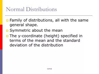
Normal Distributions. Normal Distribution. f(y) = E[Y] = μ and Var[Y] = σ 2. f(y). y. Normal Distribution. Characteristics Bell-shaped curve - < y < + μ determines distribution location and is the highest point on curve Curve is symmetric about μ

E N D
Normal Distribution f(y) = E[Y] = μ and Var[Y] = σ2 f(y) y G. Baker, Department of Statistics University of South Carolina; Slide 2
Normal Distribution • Characteristics • Bell-shaped curve • - < y < + • μ determines distribution location and is the highest point on curve • Curve is symmetric about μ • σ determines distribution spread • Curve has its points of inflection at μ + σ G. Baker, Department of Statistics University of South Carolina; Slide 3
Normal Distribution σ σ σ σ σ μ G. Baker, Department of Statistics University of South Carolina; Slide 4
Normal Distribution n(μ = 5, σ = 1) n(μ = 0, σ = 1) f(y) y G. Baker, Department of Statistics University of South Carolina; Slide 5
Normal Distribution n(μ = 0,σ = 0.5) f(y) n(μ = 0,σ = 1) y G. Baker, Department of Statistics University of South Carolina; Slide 6
Normal Distribution n(μ = 5, σ = 0.5) n(μ = 0, σ = 1) f(y) y G. Baker, Department of Statistics University of South Carolina; Slide 7
68-95-99.7 Rule 0.997 0.95 0.68 µ µ-3σ µ-2σ µ-1σ µ+1σ µ+2σ µ+3σ μ + 1σ covers approximately 68% μ + 2σ covers approximately 95% μ + 3σ covers approximately99.7% G. Baker, Department of Statistics University of South Carolina; Slide 8
Earthquakes in a California Town Since 1900, the magnitude of earthquakes that measure 0.1 or higher on the Richter Scale in a certain location in California is distributed approximately normally, with μ = 6.2 and σ = 0.5, according to data obtained from the United States Geological Survey. G. Baker, Department of Statistics University of South Carolina; Slide 9
Earthquake Richter Scale Readings 34% 34% 2.5% 2.5% 13.5% 13.5% 5.2 5.7 6.2 6.7 7.2 68% 57 159 95% G. Baker, Department of Statistics University of South Carolina; Slide 10
Approximately what percent of the earthquakes are above 5.7 on the Richter Scale? 34% 34% 2.5% 2.5% 13.5% 13.5% 5.2 5.7 6.2 6.7 7.2 68% 95% G. Baker, Department of Statistics University of South Carolina; Slide 11
The highest an earthquake can read and still be in the lowest 2.5% is _. 34% 34% 2.5% 2.5% 13.5% 13.5% 5.2 5.7 6.2 6.7 7.2 68% 95% G. Baker, Department of Statistics University of South Carolina; Slide 12
The approximate probability an earthquake is above 6.7 is ______. 34% 34% 2.5% 2.5% 13.5% 13.5% 5.2 5.7 6.2 6.7 7.2 68% 95% G. Baker, Department of Statistics University of South Carolina; Slide 13
Standard Normal Distribution • Standard normal distribution is the normal distribution that has a mean of 0 and standard deviation of 1. n(µ = 0, σ = 1) G. Baker, Department of Statistics University of South Carolina; Slide 14
Z is Traditionally used as the Symbol for a Standard Normal Random Variable Z Y 4.7 5.2 5.7 6.2 6.7 7.2 7.7 G. Baker, Department of Statistics University of South Carolina; Slide 15
Normal Standard Normal Any normally distributed random variable can be converted to standard normal using the following formula: We can compare observations from two different normal distributions by converting the observations to standard normal and comparing the standardized observations. G. Baker, Department of Statistics University of South Carolina; Slide 16
What is the standard normal value (or Z value) for a Richter reading of 6.5?Recall Y ~ n(µ=6.2, σ=0.5) G. Baker, Department of Statistics University of South Carolina; Slide 17
Example • Consider two towns in California. The distributions of the Richter readings over 0.1 in the two towns are: Town 1: X ~ n(µ = 6.2, σ = 0.5) Town 2: Y ~ n(µ = 6.2, σ = 1). - What is the probability that Town 1 has an earthquake over 7 (on the Richter scale)? - What is the probability that Town 2 has an earthquake over 7? G. Baker, Department of Statistics University of South Carolina; Slide 18
Town 1 Town 2 Town 1: Town 2: 0.212 0.055 Z Z X Y 4.7 5.2 5.7 6.2 6.7 7.2 7.7 3.2 4.2 5.2 6.2 7.2 8.2 9.2 G. Baker, Department of Statistics University of South Carolina; Slide 19
Standard Normal 0.10 0.10 0.05 0.05 0.025 0.025 0.01 0.01 0.005 0.005 1.645 -1.645 2.326 -2.326 1.282 1.96 2.576 -2.576 -1.96 -1.282 G. Baker, Department of Statistics University of South Carolina; Slide 20
The thickness of a certain steel bolt that continuously feeds a manufacturing process is normally distributed with a mean of 10.0 mm and standard deviation of 0.3 mm. Manufacturing becomes concerned about the process if the bolts get thicker than 10.5 mm or thinner than 9.5 mm. • Find the probability that the thickness of a randomly selected bolt is > 10.5 or < 9.5 mm. G. Baker, Department of Statistics University of South Carolina; Slide 21
Inverse Normal Probabilities • Sometimes we want to answer a question which is the reverse situation. We know the probability, and want to find the corresponding value of Y. Area=0.025 y = ? G. Baker, Department of Statistics University of South Carolina; Slide 22
Inverse Normal Probabilities • Approximately 2.5% of the bolts produced will have thicknesses less than ______. 0.025 Z Y ? G. Baker, Department of Statistics University of South Carolina; Slide 23
Inverse Normal Probabilities • Approximately 2.5% of the bolts produced will have thicknesses less than ______. G. Baker, Department of Statistics University of South Carolina; Slide 24
Inverse Normal Probabilities • Approximately 1% of the bolts produced will have thicknesses less than ______. 0.01 Z Y ? G. Baker, Department of Statistics University of South Carolina; Slide 25
Inverse Normal Probabilities • Approximately 1% of the bolts produced will have thicknesses less than ______. G. Baker, Department of Statistics University of South Carolina; Slide 26