Download

1 / 54
540 likes | 677 Views
This paper investigates the bidimensionality framework in graph theory, focusing on its implications for solving NP-hard problems efficiently on planar and minor-free graphs. It outlines the significance of graph minors theory and presents new exact, parameterized, and approximation algorithms, emphasizing the Dominating Set problem as a case study. Key results include the development of preprocessing techniques and the introduction of treewidth bounds for bidimensional problems, leading to faster algorithms. The work extends existing methodologies to larger graph classes, paving the way for future research in the area.

E N D
Bidimensionality (Revised) Daniel Lokshtanov Based on joint work with Hans Bodlaender ,Fedor Fomin,Eelko Penninkx, Venkatesh Raman, Saket Saurabh and Dimitrios Thilikos
Background Most interesting graph problems are NP-hard on general graphs. Often input graphs are planar or almost planar. Can this be used to give efficient algorithms? Most interesting graph problems remain NP-hard on planar graphs.
Are planar graphs as hard as general graphs? On planar graphs many problems admit: • Faster exact algorithms. • Faster parameterized algorithms. • Good preprocessing rules (kernels). • Better approximation algorithms.
Bidimensionality [DFHT] A framework that gives fast exact algorithms, paramterized algorithms, kernels and approximation schemes for problems on planar graphs. Main tool: Graph Minors theory of Robertson and Seymour. Extends to larger classes of graphs.
Problems considered Input:G Max / Min:κ(G,S) (S ⊆ V(G) / S ⊆ E(G)) Subject to:φ(G,S) Technical note: we demand that κ(G,S) ≤ |S| and that κ(G,OPT) = |OPT|. Value of optimal solution on G = π(G).
Minors and Contractions H is a minor of G (H ≤mG)if H can be obtained from G by a sequence of edge contractions, edge deletions and vertex deletions. H is a contraction of G (H ≤c G) if H can be obtained from G by a sequence of edge contractions.
grids and Γammas g4 Γ4
Bidimensionality A problem Π is (minor)-bidimensional if: • If H ≤m G then π(H) ≤ π(G). • There is a constant c such that π(gt) ≥ ct2. A problem Π is contraction-bidimensional if: • If H ≤c G then π(H) ≤ π(G). • There is a constant c such that π(Γt) ≥ ct2.
Examples of Bidimensional problems • Vertex Cover, Feedback Vertex Set, Longest Path and Cycle Packing are minor-bidimensional. • Dominating Set, Connected Vertex Cover and Independent Set are contraction-bidimensional.
Facts about Treewidth • Many graph probems can be solved in 2O(tw(G))n time. • If H ≤m G then tw(H) ≤ tw(G). • The treewidth of gk is k. • Every graph G has abalanced separatorof size tw(G). • On H-minor free graphs, treewidth is constant factor approximable.
Excluded Grid Theorem Theorem [RS]: For every fixed graph H there is a constant c such that any graph G which excludes H as a minor contains gc*tw(G) as a minor.
Excluded Γamma Theorem Theorem [FGT]: For every fixed apex graph H there is a constant c such that any graph G which excludes H as a minor contains Γc*tw(G) as a contraction.
Parameter-treewidth bound Lemma [Parameter-treewidth bound]: For every bidimensional problem Πthere is a constant c such that for anyplanar graph G,tw(G) ≤ cπ(G)1/2 Proof:By excluded grid theorem, gc*tw(G) ≤m G.SinceΠis bidimensional, π(gc*tw(G)) ≥ c’tw(G)2. Since Πis minor closed, π(G) ≥ c’tw(G)2.
Algorithm on planar graphs Constant-factor approximate treewidth. Output a decomposition of width t =O(π(G)1/2). Solve problem in 2O(t)n (or tO(t)n) time. Total time taken is 2π(G)1/2n (or π(G)π(G)1/2n).
More general graph classes Note: The only place we used planarity was for the excluded grid theorem. So results hold on H-minor-free graphs for minor-bidimensional problems and apex-minor-free graphs for contraction-bidimensional problems.
Exercise 1: Prove: For any fixed H, d,if G is H-minor-freeandhas a set X such that tw(G \ X) ≤ d then tw(G) ≤ d + O(|X|1/2). Soln: Vertex deletion into treewidth d graphs is minor closed and at least (t/(d+1))2 on gtgrids.
Separability Want: EPTASes for all bidimensional problems on (apex)-minor-free graphs. Can’t handle Longest Path. Parameter-treeewidth bound is not enough, but ”almost enough”. (1+ε)-approximation in f(ε)poly(n) time.
Separability A problem Π is separable* if for any partition of V(G) into L, S, R such that there is no edge from L to R, and optimal solution OPT ⊆ V(G): -π(G \ R) ≤ κ(G \ R, OPT \ R) + O(|S|) -π(G \ L) ≤ κ(G \ L, OPT \ L) + O(|S|) *For contraction-bidimensional problems a slightly different definition is used.
Excercise 2 Show that Vertex Cover is separable. Solution:OPT \ R is a feasible solution for G[L ∪ S]. Hence π(G \ R) ≤ |OPT \ R|.
Exercise 3: Show that Independent Set is separable. Solution: Let OPT be a maximum independent set of G. Suppose π(G \ R) > |OPT \ R| + |S|. Then π(G[L]) > |OPT \ R| Then G has an independent set of size: π(G[L]) + |OPT ∩ R| > |OPT \ R| + |OPT ∩ R| =|OPT|.
Decomposition Lemma Lemma: For any minor-bidimensional, separable problem Π on H-minor-free graphs, there is a function f : N N and polynomial time algorithm that given G and ε > 0 outputs a set X such that • |X| ≤ επ(G) • tw(G \ X) ≤ f(ε).
Exercise 4: Assume Feedback Vertex Set (FVS)is minor-bidimensional,and separable. Give an EPTAS for FVS on H-minor-free graphs using the decomposition lemma. Solution: For a fixed ε and given G find X. Solve FVS optimally on G \ X in g(ε)n time. Add X to the solution. Solution size ≤ (1+ε)π(G).
Decomposition’Lemma Lemma: For any contraction-bidimensional, separable problem Π on apex-minor-free graphs, there is a function f : N N and polynomial time algorithm that given G and ε> 0 outputs a set X such that • |X| ≤ επ(G) • tw(G \ X) ≤ f(ε).
Exercise 5: Assume Dominating Set (DS)is minor-bidimensional,and separable. Give an EPTAS for DSon apex-minor-free graphs using the decomposition’lemma. Solution: For a fixed ε and given G find X. Mark N(X). Find a smallest set S in G\X that dominates all unmarked vertices of G\X. Now S ∪ X is a DS of G of size ≤ (1+ε)π(G).
Balanced Separator Lemma For any graph G of treewidth t and vertex set X there is a partition of V(G) into L, S, R such that: • There is no edge between L and R • The separator S is small; |S| ≤ t. • The separator is balanced;|X ∩ L| ≤ 2|X|/3 and |X ∩ R| ≤ 2|X|/3
Weak, Non-constructive, Decomposition Lemma WNDL: For any minor-bidimensional, separable problem Π on H-minor-free graphs, there is a constant c such that any instance G has a vertex set X such that • |X| ≤ cπ(G) • tw(G \ X) ≤ c.
WNDL Proof • By parameter-treewidth bound, there is a constant d such that tw(G) ≤ dπ(G)1/2. • Let T(k) be the smallest number t such that any H-minor free graph G with π(G) = k contains a set X of size t such that tw(G \ X) ≤ d. • Need to prove T(k) = O(k). • Base Case: T(1) = 0 since tw(G) ≤ dπ(G)1/2 ≤ d.
WNDL recurrence Let Z be an optimal solution in G, then k=|Z|=π(G). Now, tw(G) ≤ dk1/2. Balanced Separator Lemma applied to G,Z yields decomposition of V(G) into (L, S, R) such that |S|≤ dk1/2 , L ∩ Z ≤ 2|Z|/3, R ∩ Z ≤ 2|Z|/3.
WNDLrecurrence Since Π is separable:π(G \ R) ≤ κ(G \ R, Z \ R) + O(k1/2) ≤ |Z\R|+ O(k1/2) G\R has a set XL of size T(|Z\R|+ O(k1/2) ) such that tw((G\R)\XL) ≤ d. G\Lhas a set XRof size T(|Z\L|+ O(k1/2) ) such that tw((G\L)\XR) ≤ d.
WNDLrecurrence X = XL ∪ XR ∪ S is a set of size T(|X\R|+ O(k1/2) ) + T(|X\L|+ O(k1/2) ) + O(k1/2) such that tw(G \ X) ≤ d. Observe: |X\R| + |X\L| ≤ |X| + |S|.
WNDLrecurrence T(k) ≤ T(⍺k + O(k1/2)) + T((1-⍺)k + O(k1/2)) + O(k1/2) ...where 1/3 ≤ ⍺ ≤ 2/3. This solves to T(k) = O(k).
Breathe Break Questions?
Scaling Lemma For any H and c there is a polynomial time algorithm and a function f : N Nthat given a H-minor free graph G, a set X such that tw(G\X) ≤ c, and ε > 0 outputs a set X’ of size ε|X| such that for any component C of G \ X’ • |C ∩ X| ≤ f(ε) • |N(C)| ≤ f(ε) Implies tw(G[C]) ≤ f’(ε)
Proof Idea for Scaling Lemma For a fixed γ let Tγ(k) be the smallest integer t such that any G with X such that |X|≤ k and tw(G\X) ≤ d contains a set X’ of size ≤ t such that for any component C of G \ X’ • |C ∩ X| ≤ γ • |N(C)| ≤ γ
Proof Idea for Scaling Lemma For every γ > d prove that Tγ(k) ≤ g(γ)k where g(γ) 0 as γ ∞. Prove Tγ(k) ≤ g(γ)k using balanced separation as in the proof of WNDL.
Recurrence for Scaling Lemma Tγ(γ) = 0 Tγ(k) ≤ Tγ(⍺k + O(k1/2)) + Tγ((1-⍺)k + O(k1/2)) + O(k1/2) ...where 1/3 ≤ ⍺ ≤ 2/3. See board Thus Tγ(k) ≤ g(γ)k but what is lim g(γ) when γ ∞?
Analyzing g(γ) cheat: set ⍺ = ½ and move lower order terms outside function calls. Tγ(γ) = 0 Tγ(k) ≤ 2Tγ(½k) + O(k½)
Analyzing g(γ) Tγ(γ) = 0 Tγ(k) ≤ 2Tγ(½k) + O(k½) 20 *(½0k)½ = 20/2k½ 21 *(½1k)½ = 21/2k½ 22 *(½2k)½ = 22/2k½ 23 *(½3k)½ = 23/2k½
Making Proof of Scaling Lemma constructive Proof naturally makes a divide and conquer algorithm for constructing X’ from G, X and ε. Only computationally hard step is computing treewidth. Can be constant-factor approximated instead since G is H-minor-free.
What we have, what we want Have:Weak Nonconstructive Decomposition Lemma and Scaling Lemma If we could make WNDL constructive, we would be done! Want: Constant factor approximation of ”treewidth-d deletion” on H-minor free graphs.
Protrusion Lemma For every H, d, there are constants c such that if G is H-minor-free and tw(G)>d then there is a vertex set C such that: • d < tw(G[C]) ≤ c • N(C) ≤ c Proof: Let X be smallest set such that tw(G)<d. Apply Scaling Lemma on X with ε=½. Set c=f(½). Since X’ < X some component C of G\X’has tw(G[C]) > d.
Approximation algorithm forTreewidth-d deletion Let c be as in Protrusion Lemma. While tw(G) > d: Find a vertex set C such that d < tw(G[C]) ≤ c and N(C) ≤ c. Find best treewidth-d-deletion XC in G[C]. Add Xc and N(C) to X. G G \ (C ∪ N(C)) Output X
Approximation Ratio We deletedX1, X2, X3.... Xt ≤ OPT N(C1), N(C2) ... N(Ct) ≤ ct Each Ci contains a vertex from OPT so t ≤ |OPT|. Hence |X| ≤ (c+1)|OPT|
Proof of Decomposition Lemma By WNDL there exists a treewidth d-deletion of size O(π(G)). By approximation we can find a treewidth treewidth d-deletion X of size O(π(G)). By Scaling Lemma we can turn X into a treewidth-f(ε) deletion set X’ of size ε|X|. Choosing ε small enough we get |X’| ≤ επ(G).
Approximation - recap Saw a decomposition lemma for bidiemsional, separable problems on H-minor-free graphs and how it can be used to give EPTAS’es for many problems on H-minor free graphs