Bidimensionality and Approximation Algorithms
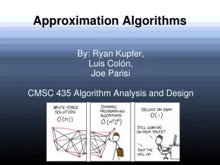
Bidimensionality and Approximation Algorithms. Mohammad T. Hajiaghayi UMD. r. r. Dealing with Hard Network Design Problems. Main (theoretical) approaches to solve NP-hard problems: Special instances: Planar graphs (fiber networks in ground), etc.


Bidimensionality and Approximation Algorithms
E N D
Presentation Transcript
Bidimensionality and Approximation Algorithms Mohammad T. Hajiaghayi UMD r r
Dealing with Hard Network Design Problems • Main (theoretical) approaches to solve NP-hard problems: • Special instances: Planar graphs (fiber networks in ground), etc. • Approximation algorithms (PTAS):Within a factor C of the optimal solution (PTAS if C= 1+ ε for arbitrary constant ε) • Fixed-parameter algorithms:Parameterize problem by parameter P(typically, the cost of the optimal solution)and aim for f(P) nO(1) (or even f(P) + nO(1)) • We consider all above in Bidimentionality and aim for general algorithmic frameworks
Overview • For any network design problem in a large class (“bidimensional”) • Vertex cover, dominating set, connected dominating set, r-dominating set, feedback vertex set, TSP, k-cut, Steiner tree, Steiner forest, multiway cut,… • In broad classes of networks generalizing planar networks (most “minor-closed” graph families) • We Obtain (in a series of more than 25 papers): • Strong combinatorial properties • Fixed-parameter algorithms • Often subexponential: 2O(√k) nO(1) where k=|OPT| • Approximation algorithms • Often PTASs (1+ ε approx): f(1/ε) nO(1)
Beyond Planar Graphs • A graph G has a minor HifH can be formed by removing and contracting edges of G * delete G H minor of G contract • Otherwise, if G exclude H as a minor is called an H-minor-free graph • For example, planar graphs are bothK3,3-minor-free and K5-minor-free
Graph Minor Theory[Robertson & Seymour 1984–2004] • Seminal series of ≥ 20 papers • Powerful results on excluded minors: • Every minor-closed graph property(preserved when taking minors)has a finite set of excluded minors[Wagner’s Conjecture] • Every minor-closed graph propertycan be decided in polynomial time • For fixed graph H, graphs minor-excluding H have a special structure: drawings onbounded-genus surfaces + “extra features”
Treewidth[GM2—Robertson & Seymour 1986] • Treewidthof a graph is the smallest possible width of a tree decomposition • Tree decompositionspreadsout each vertex as aconnected subtree of acommon tree, such thatadjacent vertices haveoverlapping subtrees • Width= maximum overlap − 1 • Treewidth 1 tree; 2 series-parallel; … Treedecomposition Graph (width 3)
Treewidth Basics • Many fast algorithms for NP-hard problems on graphs of small treewidth • Typical running time: 2O(treewidth) nO(1) • Computing treewidth is NP-hard • Computable in 22O(treewidth) n time, includinga tree decomposition [Bodlaender 1996] • O(1)-approximable in 2O(treewidth) nO(1) time, including a tree decomposition [Amir 2001] • O(√lg opt)-approximable in nO(1) time[Feige, Hajiaghayi, Lee 2004] (using a new framework for vertex separators based on embedding with minimum average distortion into line)
Treewidth Basics • Many fast algorithms for NP-hard problems on graphs of small treewidth • Typical running time: 2O(treewidth) nO(1) • Computing treewidth is NP-hard • Computable in 22O(treewidth) n time, includinga tree decomposition [Bodlaender 1996] • O(1)-approximable in 2O(treewidth) nO(1) time, including a tree decomposition [Amir 2001] • 1.5-approximation for planar graphs and single-crossing-minor-free graphs [EDD,MTH,NN,PR,DMT] • O(|V(H)|^2)-approximable in nO(1) time in H-minor-free graphs [Feige, Hajiaghayi, Lee 2004]
Bidimensionality (version 1) • Parameter k is minor-bidimensional if • Closed under minors:k does not increasewhen deleting orcontracting edges and • Large on grids:For the r r grid, k = Ω(r2) and more generally Ω(f(r)) v w v w v w delete contract r r
Example 1: Vertex Cover • k = minimum number of vertices required to cover every edge (on either endpoint) • Closed under minors: v w v w v w v w v w cover v w v w delete contract still a cover (only fewer edges) still a cover,possibly 1 smaller
Example 1: Vertex Cover • k = minimum number of vertices required to cover every edge (on either endpoint) • Large on grids: • Matching of size Ω(r2) • Every edge must be coveredby a different vertex v w v w v w v w cover r r
Bidimensionality (version 2) • Parameter k is contraction-bidimensional if • Closed under contractions:k does not increasewhen contracting edges and • Large on a grid-like graph:For naturally triangulatedr r grid graphs, k = Ω(r2) v w v w contract
Example 2: Dominating Set • k = minimum number of vertices required to cover every vertex or its neighbor • Large on grids: • Ω(r2) vertex-disjoint cycles • Every cycle must be coveredby a different vertex … v w v w v w v w cover u u u u r r
Example 2: Dominating Set • k = minimum number of vertices required to cover every vertex or its neighbor • Closed under contraction but not minor: v w … v w v w v w v w cover u u u u v w v w delete contract • Not necessarily • a cover anymore still a cover,possibly 1 smaller
Contraction-Bidimensional Problems • Minimum maximal matching • Face cover (planar graphs) • Dominating set • Edge dominating set • R-dominating set • Connected … dominating set • Unweighted TSP tour • Chordal completion (fill-in) v w v w contract
Bidimensional RelateParameter & Treewidth & • Theorem 1: If a parameter k isbidimensional, then it satisfiesparameter-treewidth bound treewidth = O(√k)in any graph family excluding some minor[Demaine, Fomin, Hajiaghayi, Thilikos, JACM 2005; Demaine & Hajiaghayi, Combinatorica 2010] • Proof sketch:Large treewidth very large grid [minor theory] very large k [bidimensional]
Bidimensional Subexponential FPT & • Theorem 2:If a parameter k is • bidimensional, and • fixed-parameter tractable on graphs of bounded treewidth: h(treewidth) nO(1) time then it has a subexponential fixed-parameter algorithm: h(√k) nO(1) timein any graph family excluding some minor • Typically 2O(√k) nO(1) time (h(w) = 2O(w)) [Demaine, Fomin, Hajiaghayi, Thilikos 2004; Demaine & Hajiaghayi 2005] • Proof sketch:Run bounded-treewidth algorithm (tw = O(√k)) [If (approx.) treewidth is large, answer NO]
Bidimensional Subexponential FPT v w v w u • Corollary 1:Vertex cover and feedback vertex set have subexponential fixed-parameter algorithms: 2O(√k) nO(1) time in any graph family excluding some minor[Demaine, Fomin, Hajiaghayi, Thilikos 2004; Demaine & Hajiaghayi 2005] • Previously known for vertex cover (and some other problems) on planar graphs [Alber et al. 2002; Kanj & Perković 2002; Fomin & Thilikos 2003; Alber, Fernau, Niedermeier 2004; Chang, Kloks, Lee 2001; Kloks, Lee, Liu 2002; Gutin, Kloks, Lee 2001]
Bidimensional PTAS & • Theorem 3:If a parameter is • bidimensional, • fixed-parameter tractable on graphs of bounded treewidth: h(treewidth) nO(1) time, • O(1)-approximable in polynomial time, and • satisfies the “separation property” then it has an PTAS:(1+ε)-approximation in h(O(1/ε)) nO(1) time in any graph family excluding some minor[Demaine & Hajiaghayi, SODA’05]
Bidimensional PTAS v w v w u • Corollary 3: Vertex cover and feedback vertex set have PTASsin any graph family excluding some minor[Demaine & Hajiaghayi 2005] • Previously known for vertex cover (and many, many other problems) on planar graphs • E.g., feedback vertex set result is new,even for planar graphs
Consequence: Separator Theorem • Theorem:[Demaine, Fomin, Hajiaghayi, Thilikos 2004; Demaine & Hajiaghayi 2005]For every bidimensional parameter P, treewidth(G) ≤ √P(G) • Apply to P(G) = number of vertices in G • Corollary: For any fixed graph H, every H-minor-free graph has treewidth O(√8n)[Alon, Seymour, Thomas 1990; Grohe 2003] • Corollary: 1/3-2/3 separators, size O(√n) (A vertex set whose removal leaves no component of size greater than 2n/3)
Application to Independent Set (Lipton-Tarjan 1980) • Independent Set: a set of vertices with no edges in between • Note that OPT is at least n/4 since planar graphs are 4-colorable • For PTAS break each component of greater than εn (=log n) and ignore separator vertices • Solve each component individually and take their union as the final solution • Consider a laminar family: level 0 are leaves
Application to Ind. Set (cont’d) • The maximum number of levels is at most log3/2 n • Say C is the union of all separator (ignored) vertices. • Note that l<= n/ ((3/2)i-1ε n) since the size of a level I component is at least (3/2)i-1ε n • Let ε= log n/n, so εn= log n (and thus we can solve each component individually in 2log n= n time) • So the total number of ignored vertices is at most n/ (√ log n)< ε n/4<= ε OPT (In each component we are not worse than OPT)
Polynomial-TimeApproximation Schemes • Separator approach [Lipton & Tarjan 1980]gives PTASs only when OPT (after kernelization) can be lower bounded in terms of n (typically, OPT = Ω(n)) • Examples: Various forms of TSP[Grigni, Koutsoupias, Papadimitriou 1995; Arora, Grigni, Karger, Klein, Woloszyn 1998; Grigni 2000; Grigni & Sissokho 2002] • Parameter-treewidth bounds give separators in terms of OPT, not n
Polynomial-TimeApproximation Schemes • Theorem: [Demaine & Hajiaghayi 2005](1+ε)-approximation with running time h(O(1/ε)) nO(1) for any bidimensional optimization problem that is • Computable in h(treewidth(G)) nO(1) • Solution on disconnected graph = union of solutions of each connected component • Given solution to G − C, can compute solution to G at an additional cost of ± O(|C|) • Solution S of G induced on connected component X of G−C has size |S X| ± O(|C|)
Polynomial-TimeApproximation Schemes • Corollary: [Demaine & Hajiaghayi 2005] • PTAS in H-minor-free graphs for feedback vertex set, face cover, vertex cover, minimum maximal matching, and related vertex-removal problems • PTAS in apex-minor-free graphs for dominating set, edge dominating set, R-dominating set, connected … dominating set, clique-transversal set • No PTAS previously known for, e.g., feedback vertex set or connected dominating set, even in planar graphs
… … … … Graph Decomposition … … … … [Lipton & Tarjan 1980; …]
Simplifying Graph Decomposition[Demaine, Hajiaghayi, Kawarabayashi, SODA 2010] • Theorem: OddH-minor-free graphs can have their vertices or edges partitioned into twopieces such that each induced graph has bounded treewidth • Previously for planar graphs [Baker 1994],apex-minor-free [Eppstein 2000],H-minor-free [DeVos et al. 2004; Demaine, Hajiaghayi, Kawarabayashi, FOCS’05]
Example: Graph Coloring • Chromatic number: Use fewest colorsto color the vertices of a graph such that no two equal colors connected by an edge • Classic NP-hard problem • Inapproximable within n1−ε unless ZPP = NP Martin Gardner,April 1, 1975
Example: Graph Coloring[Demaine, Hajiaghayi, Kawarabayashi 2005/2010] • 2-approximation for chromatic numberin odd-H-minor-free graphsusing decomposition into twobounded-treewidth pieces: General graphs:Inapprox. within n1−ε unlessZPP = NP
Simplifying Graph Decompositions[DeVos et al. 2004; Demaine, Hajiaghayi, Kawarabayashi 2005] • Generalization to k pieces:H-minor-free graphs can have their vertices or edges partitioned into kpieces such that deleting any one piece results in bounded treewidth • Useful for PTASs for minor-closed properties (where k ~ 1/ε) • (Not true for odd-minor) • Application: e.g. PTAS for MaxCut
Many Problems Closed Under Contractions but not Deletions • Dominating set • Edge dominating set • R-dominating set • Connected … dominating set • Face cover (planar graphs) • Minimum maximal matching • Chordal completion (fill-in) • Traveling Salesman Problem • …
Contraction Decomposition[Demaine, Hajiaghayi, Kawarabayashi, STOC’11] • Theorem: H-minor-free graphs can have their edges partitioned into k pieces such that contractingany one piece results in bounded treewidth • Polynomial-time algorithm • Previously known for planar [Klein 2005, 2006], bounded-genus [Demaine, Hajiaghayi, Mohar 2007], apex-minor-free [Demaine, Hajiaghayi, Kawarabayashi 2009]
Applications • Lots of applications via a general theorem,e.g. • Corollary 1: PTAS for Traveling Salesman Problem in weighted H-minor-free graphs[Demaine, Hajiaghayi, Kawarabayashi 2011] solving an open problem of[Grohe 2001] • Coroallary 2: Fixed-Parameter Algorithm for k-cut and Bisection on planar graphs and H-minor-free graphs [Demaine, Hajiaghayi, Kawarabayashi 2011] solving an open problem of [Downey, Estivill-Castro, Fellows 2003]
Application to TSP • Corollary: PTAS for Traveling Salesman Problem in weighted H-minor-free graphs[Demaine, Hajiaghayi, Kawarabayashi 2011] • Existing bounded-treewidth algorithm[Dorn, Fomin, Thilikos 2006] • Existing spanner [Grigni, Sissokho 2002] • Decontraction: • Euler tour(cost ≤ 2 weight)+ perfect matching on odd-degree vxs (cost ≤ weight)
Graph TSP History • PTAS for unweighted planar[Grigni, Koutsoupias, Papadimitriou 1995] • PTAS for weighted planar[Arora, Grigni, Karger, Klein, Woloszyn 1998] • Linear PTAS for weighted planar [Klein 2005] • QPTAS (n(1/ε) O(log log n) time) for weighted bounded-genus / unweighted H-minor-free [Grigni 2000] • PTAS for weighted bounded genus[Demaine, Hajiaghayi, Mohar 2007] • PTAS for unweighted apex-minor-free [Demaine, Hajiaghayi, Kawarabayashi 2009] • PTAS for weighted H-minor-free [DHK 2011]
Application Beyond TSP • Corollary: PTAS for minimum-weightc-edge-connected submultigraphin H-minor-free graphs[Demaine, Hajiaghayi, Kawarabayashi 2011] • Previous results: • PTASs for 2-edge-connected in planar graphs[Klein 2005] (linear)[Berger, Czumaj, Grigni, Zhao 2005][Czumaj, Grigni, Sissokho, Zhao 2004] • PTAS for c-edge-connected in bounded-genus graphs [Demaine, Hajiaghayi, Mohar 2007]
Fixed-Parameter Algorithmic Applications: k-cut • k-cut: Remove fewest edges to makeat least k connected components • FPT in H-minor-free graphs: • Average degree cH = O(H lg H ) • OPT ≤ cH k • Contraction decomposition with cH k + 1 layers avoids OPT in some contraction • Solve in 2Õ(k) n + nO(1) time • Generalization to arbitrary graphs [Kawarabayashi & Thorup 2011] √‾‾‾
Proof Sketch • H-minor-free graph = “tree” of“almost-embeddable graphs” [Graph Minors] • Each almost-embeddable graph has contraction decomposition: • Bounded genus done • Apices easy:increase treewidthof anything by O(1) • Vortices similar [Demaine, Hajiaghayi, Mohar2007]
Radial Coloring for Bounded Genus • Color edge at radial distance r as r mod k • Radial graph ≈ primal graph + dual graph • Any k consecutive layers have bounded treewidth, provided first k do
Contraction Decomposition[Demaine, Hajiaghayi, Kawarabayashi 2011] • Theorem: H-minor-free graphs can have their edges partitioned into k piecessuch that contractingany one piece results in bounded treewidth • Polynomial-time algorithm • Seems a powerful tool for approximation & fixed-parameter algorithms • Let’s find more applications!
Graph Minors[Robertson&Seymour 1983–2004] in ≥ 20 papers … …
NonconstructiveGraph Minors • Theorem: Every H-minor-free graph can be writtenas a tree of graphs joinedalong f(H)-size cliques • Each term is a graph that can be almost embedded into a bounded-genus surface(f(H) “vortices” and “apices”) [GM16: Robertson & Seymour 2003]
ConstructiveGraph Minors • Theorem: Every H-minor-free graph can be writtenas a tree of graphs joinedalong f(H)-size cliques • Computable in nf(H) time[Demaine, Hajiaghayi, Kawarabayashi, FOCS 2005] • Weaker form in f(H) nO(1) time[Dawar, Grohe, Kreutzer 2007]
Grid Minors • Every H-minor-free graph of treewidth≥ f(H) r has an r r grid minor[Demaine & Hajiaghayi, SODA 2005, Combinatorica 2010] • Previous bounds exponential in r and H[GM5—Robertson & Seymour 1986;Robertson, Seymour, Thomas 1994; Reed 1997;Diestel, Jensen, Gorbunov, Thomassen 1999] • Open: What is f(H)? • Ω(√|V(H)| lg |V(H)|) • Conjecture: |V(H)|O(1) or even O(|V(H)|)
Beyond Bidimensionality • Nontrivial weights • Min-weight k disjoint paths? • Directed networks (with Rajesh) • Useful notion of treewidth? • Subset problems (with Rajesh and Marek) • Steiner tree, subset TSP, etc. have PTASsup to bounded-genus graphs [Borradaile, Mathieu, Klein 2007; Borradaile, Demaine, Tazari 2009] • Steiner forest has PTAS in planar graphs[Bateni, Hajiaghayi, Marx 2010] • Wanted: A more general framework k = 3