Download
1 / 36
370 likes | 457 Views
Dive into the world of astronomical observations with a focus on telescopes, detectors, images, and spectroscopy. Learn about telescope types, imaging techniques, detectors, and more fundamental aspects of observing the cosmos.

E N D
Astronomical observations • Telescopes • Instruments and observations • Detectors • Astronomical images • Spectroscopy
Telescopes • End of 16th Century: the first refracting telescopes are built in the Netherlands • 1609: Galileo builds his own telecope and turns it towards the sky • 1671: Newton builds the first reflecting telescope Galileo observing the sky Replica of the first Newton’s telescope
Telescopes - 2 Telescope types • Refracting: − based upon lenses → size limited to ~1 m chromatic aberrations • Reflecting: − based upon mirrors → light does not go through glass but partial obstruction
Telescopes - 3 Main characteristics of a telescope • Diameter of primary mirror d → collecting surface • Focal distance F → scale of image in focal plane: F /206235(in mm/arcsec if F in mm) • Aperture ratio F / d → optical speed (flux concentration) • Angular resolution θ = 1.22 λ / d for a circular aperture of diameter d F d
Telescopes - 4 Other telescope characteristics • Image quality − angular diameter of circle in which a given fraction of the light fom a point source is concentrated • Field − region of the focal plane which is lit or: − region of the focal plane where image quality is adequate • Focal plane curvature (ex: Schmidt telescope – wide field but curved focal plane)
Telescopes - 5 Types of foci Several possibilities: (1) detector at prime focus (2) a secondary mirror deflects the light beam towards another focus – Newton – Cassegrain – Coudé – Nasmyth
Telescopes - 6 Equatorial mount In order for the telescope to keep pointing towards a celestial object, Earth’s rotation must be compensated → telescope mounted on 2 axes: – a 1st axis parallel to Earth’s rotation axis (polar axis) – a 2d axis perpendicular to the latter (declination axis) → polar axis rotates (360° per sidereal day)
Telescopes - 7 Altazimutal mount Thanks to computers, one can go back to a simpler mount: – a 1st vertical axis (azimut axis) – a 2d horizontal axis (elevation axis) Advantages: – simpler, more compact → cheaper – axes parallel and perpendicular to gravity → more stable → system adopted for the large modern telescopes
Instruments and observations The large majority of astronomical observations consist in analyzing the photons collected by the telescope: • Photometry: number of photons per unit of time in a given spectral band (→ filters) • Imaging: photometry + number of photons as a function of angle • Spectroscopy: number of photons as a function of energy (→ of wavelength λ) • Polarimetry: number of photons as a function of polarisation + Combination of ≠ techniques (ex: spectropolarimetry)
Photometry • Let F0(λ) be the flux emitted at the surface of an object of radius R at a distance d from the observer • As it travels towards the observer, the flux is reduced by: – geometric dilution → received flux F(λ) = F0(λ) R2/d2 – interstellar absorption by dust – absorption in Earth atmosphere (if ground-based telescope) • It is then modified by the instrument itself: – telescope (mirrors) – filter – detector
Detectors • The first detector used was the human eye (or rather its retina) Drawbacks: – short integration time (~ 1/15th of a second) – no reliable recording of the observation • Photographic emulsion brought a huge progress Advantages: – possibility of long integration times (several hours) – reliable long term recording Drawbacks: – low efficiency (~ 3% of photons are detected) – non linearity (emulsion darkening not proportional to luminous flux) – poor reproducibility
Detectors - 2 Electronic detectors Many electronic detectors start to be developed in the 70s and 80s (Reticon, Digicon…) Among them, the CCD (Charge-Coupled Device) rapidly emerges Advantages with respect to photographic emulsions: – quantum efficiency (up to > 90%) → more than a factor 30 gain! – linearity Drawbacks: – small size (a few cm2) – sensitive to cosmic rays
Detectors - 3 Photon detection in a semiconductor CCDc are based on semiconductors (generally Si) They are characterized by a valence band and a conduction band separated by a gap. E At absolute zero: – valence band is full – conduction band is empty – a photon can be absorbed and give its energy to a valence band e− that is sent into conduction band E bande de conduction e− Egap bande de valence h+
Detectors - 4 Charge collection Electrons in the conduction band are free to move inside the silicon Surface electrodes create potential wells that attract these free e− electrode V+ isolating layer silicon
Detectors - 5 charge transfer (shutter closed) charge collection (shutter open) Working of a CCD channel stops (p-doped regions) + + + electrodes silicon pixel output amplifier
Detectors - 6 CCD sensitivity Photons can be absorbed only if E > Egap Nγ ~ α (E − Egap) as long as E not too high then saturated and goes down Quantum efficiency = percentage of incident photons that are detected Quantum efficiency of a particular CCD
Detectors - 7 Photon absorption in silicon Photons penetrate deeper as λ increases Electrodes are opaque in UV electrode V+ isolating layer silicon
Detectors - 8 Improvement of sensitivity in blue and UV Thinned backside illuminated CCDs silicon isolating layer electrode V+ Refractive index of Si is high → possibility of multiple reflections at large λ→ possibility of `fringes´ if surfaces are not perfect planes
Detectors - 9 Linearity and saturation When the potential well is nearly full, free e− are much less attracted by the electrodes →non linearity followed by saturation Ne Charge transfer is also perturbed →blooming ~105 0 Nγ ~105
Detectors - 10 Parasite signals Dark current: e− excited by thermal effect → cool the CCD Cosmic ray impacts: ionizing particles crossing the CCD → a large number of e− are freed in contiguous pixels (pinned by the shape or multiple poses)
Detectors - 11 Bias, gain and readout noise Output amplifier → intrinsic internal noise (depends on electronics, readout speed) = readout noise (RON) typically a few e− Dynamic range of CCD: RON ~1 , saturation ~105 → dynamic range ~105 Analog – digital converter (ADC): transforms measured signal into a number (ADU – Analog to Digital Unit) Generally 16 bits (0 → 65535) or 32 bits Gain: g = Ne / NADU ~1 (unit: e− /ADU) Bias: additive constant to avoid negative signals (and thus loose a bit for the sign)
Detectors - 12 Possible causes: – slight size differences between pixels – dust on camera lens – non uniform lighting of the field… ideal CCD actual CCD* Observation of a flat field (*a bit exaggerated)
Astronomical images Instrumental profile Image of a point source through a circular aperture = Airy rings Δθ Seeing Ground-based observations → atmospheric turbulence If exposure time long enough → image a bit blurred
Astronomical images – 2 Angular resolution ≈ minimal angular distance between two point sources of same brightness that can be resolved ≈ FWHM (= Full Width at Half Maximum) of a point source By some misuse of language, one calls seeing the FWHM of a point source observed with a ground-based instrument Typically, seeing is ~1" (~0.5" in the best sites) FWHM
Astronomical images – 3 Signal-to-noise ratio: S/N = ratio between signal and its measurement uncertainty (noise) – in a pixel – in an astronomical object Counting of photons: obeys Poisson statistics →σ = √Ne S Sobj Ssky
Astronomical images – 4 Limiting magnitude = magnitude of faintest object that can be detected on a given exposure, with a given S/N (ex: S/N = 3)
Astronomical images – 5 Image reduction = transformation of a raw image into a scientifically useful image (reduced image) • bias subtraction (measured on zero exposure time images) • correction of interpixel nonuniformities (division by a uniform field exposure: flat field) • detection of cosmic ray impacts + `cosmetic ´correction (scientifically, the information is lost in these pixels → σ= ∞) • subtraction of sky background • computation of an image containing the intensity uncertainties σ
Spectroscopy Spectrum = quantity of light as a function of wavelength λ Spectrograph / spectrometer = instrument used to get a spectrum → based on a dispersivecomponent (decomposes light as a function of λ) Common dispersive components: prisms diffraction gratings
Spectroscopy – 2 Diffraction grating transmission or reflection β α d sinα d sinβ constructive interference if n = diffraction order d
Spectroscopy – 3 Angular dispersion: Spectral resolution (W = full width of grating): Resolving power:
Spectroscopy – 4 Position of order maxima: (grating equation) In polychromatic light: • maxima corresponding to different λ for a given n constitute the nth-order spectrum • 0th-order spectrum = white light (no dispersion) • to avoid overlap of different orders: – use a filter to select a portion of the spectrum or – cross-dispersion
Spectroscopy – 5 Cross-dispersion • high resolution → observe in high order → large order overlap • to avoid order overlap, one introduces a predisperser: prism or grating whose dispersion is perpendicular to the main grating’s order n+6 n+4 n+2 cross dispersion n n–2 n–4 n–6 main dispersion
Spectroscopy – 6 Blazed grating • main drawback of transmission grating: most of the light goes into 0th-order → lost for spectroscopy → low efficiency • solution = blazed reflection grating → most light goes into higher orders grating normal facet normal ϕ
Spectroscopy – 7 Spectrometer • Basic elements of a grating spectrometer: – entrance slit – grating – detector • Additional elements: – collimator M1 (spherical mirror) → parallel beam – camera M2 (spherical mirror) → converging beam fcoll fcam
Spectroscopy – 8 Resolution of a spectrometer • Entrance slit of width S → seen from the grating under an angle dα = S/fcoll • Grating equation: • Image of the entrance slit has a width • It corresponds to a spectral interval • With
Spectroscopy – 9 Actual resolution • Grating: • Slit: • Actual line profile = convolution of grating and slit line profiles → the broadest one dominates • In order not to loose too much light, the slit has to be matched to the size of stellar images in the telescope focal plane → resolution is generally limited by the slit width