Download
1 / 15
150 likes | 255 Views
This session covers interpreting linear models with quantitative and categorical factors, exploring effects of fertilizer and variety on paddy yields, fitting regression equations, and comparing variety means. Learn to interpret ANOVA results and model estimates for effective data analysis.

E N D
Comparing Regressions (Session 14)
Learning Objectives At the end of this session, you will be able to • understand and interpret the components of a linear model with one quantitative variable and one categorical factor • interpret output from such models • write regressions equations for each level of the categorical variable using the model estimates
Return to the Paddy example In the paddy example, consider the possible effects of fertiliser and variety together. Objective is to explore whether fertiliser or variety of both affect paddy yields. Note that the two explanatory variables (we will call them factors) being considered here are of different types, one is a quantitative variable, the other is a categorical variable.
Models with each factor in turn Previously we have fitted each variable one at a time. Thus the model with fertiliser alone is: yi =0+ 1(fert)i + i while the model with variety alone is: yij =’0+ vi + ij In models above, 0 , ’0represent constants, 1 is the slope of the line in first model and vi (i=1,2,3) represent the variety effect in 2nd model.
One model with both factors We can put the two factors together into a single model as: yij =0+ 1(fert)ij + vi + ij This model fits a regression lines with common slope for each variety, i.e. it represents three parallel lines. The intercepts of the lines are: (0 + v1), (0 + v2) and (0 + v3).
Anova results (sequential) The Residual M.S. (s2) = 0.2288. It describes the variation not explained by fertiliser and variety. How may the above results be interpreted?
Anova results (adjusted) In anova above, each term has been adjusted for the other. So S.S. for fertiliser, variety and residual do not add to the total S.S. What conclusions may be drawn from above?
Model estimates What do these results tell us?
Comparing variety means As before, comparisons with the base level can be made using the model estimates. In addition, because the results need to be adjusted for the effect of fertiliser, results again need to be reported in terms of adjusted means! These are usually calculated at the overall mean of the fertiliser variable = 1.444
Raw means and adjusted means Variety means adjusted for fertiliser effect:
Parallel lines for each variety Equations describing the regression of yield on fertiliser for each variety are: y =0+ 1 (fert) + vi y = (0+ vi) + 1 (fert) Thus for the new improved variety, y = (4.776 + 0) + 0.526 (fert) y = 4.776 + 0.526 (fert) Similarly, equations can be found for the remaining two varieties.
Model with different slopes We can put the two factors together into a single model as: yij =0 + 1(fert)ij + vi + i(fert)ij + ij This model fits regression lines with different intercepts (0 + vi), and diff. slopes (1 + i). The separate slopes are: (1 + 1), (1 + 3) and (1 + 3).
Anova with different slopes Fitting separate lines involves fitting an interaction term (see below) What are your conclusions?
Final model…. Clear from above that the added term in the model to allow for different slopes is non-significant. Hence return to the parallel lines model, i.e. y = 4.776 + 0.526(fert), for new variety y = 3.569 + 0.526(fert), for old variety y = 2.597 + 0.526(fert), for traditional
Practical work follows to ensure learning objectives are achieved…