Download
1 / 31
310 likes | 451 Views
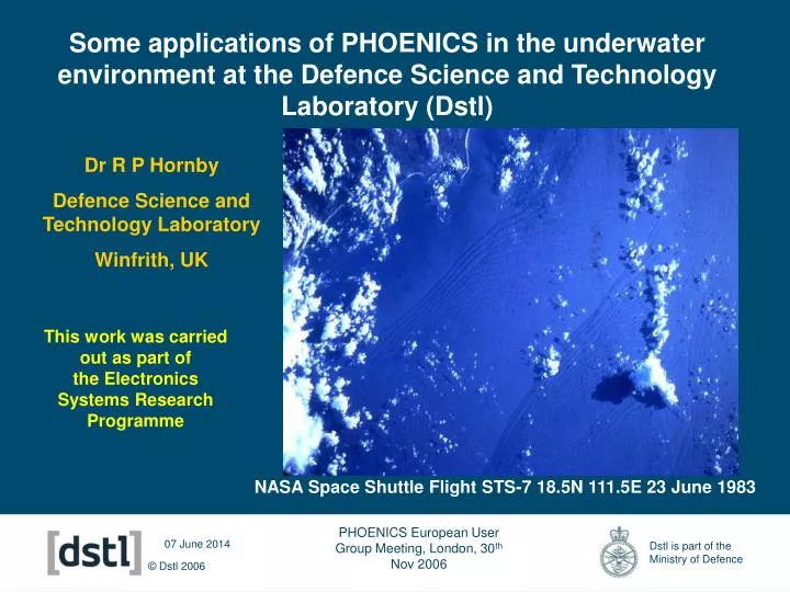
Some applications of PHOENICS in the underwater environment at the Defence Science and Technology Laboratory (Dstl). Dr R P Hornby Defence Science and Technology Laboratory Winfrith, UK. This work was carried out as part of the Electronics Systems Research Programme.

E N D
Some applications of PHOENICS in the underwater environment at the Defence Science and Technology Laboratory (Dstl) Dr R P Hornby Defence Science and Technology Laboratory Winfrith, UK This work was carried out as part of the Electronics Systems Research Programme NASA Space Shuttle Flight STS-7 18.5N 111.5E 23 June 1983 PHOENICS European User Group Meeting, London, 30th Nov 2006
Why PHOENICS? • Predicting the underwater environment is a challenging problem • Vital in assessing the performance of underwater sensors and the feasibility of maritime operations • Shelf Sea and Ocean models (UK Metrological Office) • Provide environmental information at relatively large scale • Not currently able to economically resolve the smaller scale processes • Internal wave motions • Affect water column density structure • Produce relatively large current pulses • Enhance turbulence and mixing • These models also employ a hydrostatic approximation • Restricted to processes with relatively small vertical velocities • Precludes analysis of large amplitude internal wave propagation • PHOENICS • General purpose fluid flow package solving the full equations of motion • Used to investigate these relatively small scale, but important, environmental effects
Observations of internal waves University of Delaware (US) database • Regions of most energetic Shelf Edge internal tides • UK Shelf, Bay of Biscay • China Seas • Amazon Shelf • Northwest Australian Shelf, Timor Sea • Cape Cod Grand Banks, New York Bight, Mid Atlantic Bight • Bay of Bengal, Andaman Sea • Mid-Argentine Shelf • Pakistan/Goa Shelf, Arabian Sea • Gulf of Panama • Gulf of Alaska • North Bering Sea • Regions of most energetic internal tides at straits, ridges and seamounts • Strait of Gibraltar • Strait of Messina • Strait of Malacca • Mascarene Ridge • Mid-Atlantic Ridge • Hawaian Ridge • Horseshoe seamounts (Portugal) • Hebrides Terrace, Anton Dohrn Seamounts (NW of UK) Luzon Strait, South China Sea UK Shelf
Large amplitude internal waves • Large amplitude internal waves • Prevalent where stratified ocean is forced over bathymetry • Shelf edge regions (eg UK Malin Shelf) • Straits (eg Gibraltar) • Ridges and seamounts • Amplitudes as large as 100-150m, ‘wavelength’ ~ 1000m • Phase speed ~1m/s Wave of depression Wave of elevation
Radar imaging of internal waves Adapted from Liu et al 1998; waves are travelling from right to left
UK Shelf study area Shelf Edge Study (SES) area
Left: Synthetic Aperture Radar image of SES study area Right: SES mooring marked with diamonds and labelled S700 to S140. Thermistor chain track shown as dotted line, 0000-0200 19th August 1995. ‘A’ ,’B’ mark position of lead solitons at 1136 on 20th and 21st August 1995. UK Shelf study area Light bands followed by dark bands B 300m
UK Shelf study area: internal wave profiles Malin shelf internal wave. Density (kg/m3) field (left) and horizontal velocity (m/s) field (right) at t=0s. Water depth=140m.
South China Sea • ASIAEX (Asian Seas International Acoustics Experiment) • ONR sponsored, 2001 • Orr and Mignerey (NRL, 2003) reported in situ measurements • ADCP (Acoustic Doppler Current Profiler:200, 350kHz) • Water velocity as function of depth • Acoustic backscatter from plankton, zooplankton etc or turbulence to map internal wave shape • CTD (Conductivity Temperature Depth probe) • Density structure • RADAR • Detects internal wave at distance due to backscatter from surface ‘roughness’ induced by passage of wave • Real time display allows perpendicular traverse of wave
Measurement site Asian Seas International Acoustics Experiment, 2001 Transformation, Mixing Luzon Strait Generation: Kuroshio, tidal Spreading Refraction Diffraction Reflection
Radar imaging of internal waves, South China Sea Dark bands followed by light bands as waves shoal Light bands followed by dark bands From Hsu and Liu 2000
IW ship survey Orr and Mignerey, 2003 Upslope direction (dashed line) Ship track (solid line) P Mignerey, private communication
Acoustic backscatter Orr and Mignerey, 2003 Horizontal axis is time ~70m and 40m amplitude waves in deep water, travelling from left to right
Simulation approach Malin Shelf • Computational Fluid Dynamics • Unsteady 2-D equations of motion, no Coriolis force (Ro>>1), Cartesian grid • 3rd order accurate spatial upwind scheme • 1st order implicit in time • Porosity representation for arbitrary bathymetry • Grid: dx=15m, dy=2m, dt=1.25s (Determined from previous simulations) • Source term for bed friction • Two equation k,e turbulence model with buoyancy effects • Initial waveform derived from weakly non-linear theory • Simulate internal wave propagation • 260m to 100m over 20km range • Slope gradient 1 in 125
Density structure Nmax~ 17cph Typical temperature and salinity measurements (left) and resulting averaged density profile (right).
Initial wave shape and range velocity fields 100m amplitude wave. (Left) Initial density field showing wave shape, KdV shape (dotted) and empirical KdV (solid). (Right) Initial range velocity field.
IW profiles Elevation waves appearing in 175m to 190m depth (measurements record 150m to 180m depth) (Left) CFD wave evolution for initial 70m wave and (right) 100m wave. The time interval between each profile is 1250s. The thick dashed line represents the sea bed.
IW phase speed Green Cyan Purple Red Yellow Blue ADCP record (Mignerey, private communication) marked with features used to determine wave phase speeds Variation of wave phase speed with on shelf propagation. The solid curve represents the 100m amplitude initial wave and the dashed curve the 70m amplitude initial wave. ASIAEX measurements (coloured) ; Mignerey, private communication
IW shape CFD (left) wave profile predictions for the 100m initial wave at t=21250s compared with observations (right, Orr and Mignerey, 2003) from ADCP backscatter intensity. Waves are travelling from left to right.
IW velocity field CFD(left) range velocity comparison for the 100m initial wave at t=21250s with ADCP (right, Orr and Mignerey private communication) range velocity measurements
IW kinetic energy – upslope component Total ke from ADCP Upslope ke from ADCP Kinetic energy per unit crest length in a control volume centred on the leading wave and extending 2.5km in the upstream and downstream directions (from 22.4m below the surface to 24m above the bottom). Square symbols – 7th May, triangles 8th May. ADCP upslope ke: Mignerey, private communication. Estimates (with error bar) from ADCP for just lead soliton and elevation wave GM Simulation (upslope)
Turbulent dissipation rate (Left) Log10 of the rate of dissipation of turbulent kinetic energy per unit mass at t=11250s (scale range is –9.05 to –3.79). Density contours relative to 1000 kg/m3 are superimposed to illustrate the wave shape in relation to the dissipation predictions. (Right) Gradient Richardson number plot.
Turbulent dissipation rate (Left) Log10 of the rate of dissipation of turbulent kinetic energy per unit mass at t=21250s (scale range is –9.05 to –3.84). Density contours relative to 1000 kg/m3 are superimposed to illustrate the wave shape in relation to the dissipation predictions. (Right) Gradient Richardson number plot.
Turbulent dissipation rate – elevation waves Peak dissipation rate levels ~10-4 W/kg predicted in the elevation waves
Turbulence levels • Turbulent kinetic energy integrated over a control volume 2.5km upstream and downstream of leading wave • Energy dissipation rate by turbulence in a control volume 2.5km upstream and downstream of leading wave • Energy dissipation rate and turbulence levels peak as elevation waves form
Ambient turbulence Dstl Mixed Layer Model Shelf sea -vertical profiler (UW) Oregon coast – J Moum Dstl Mixed Layer Model Open literature, various sources Elevation wave prediction
Bottom shear stress Typical shear stress distribution Maximum bed stress with range Flow distribution A bed stress ~ 2N/m**2 would lift sand type particles with diameter < ~0.1mm (Shields criterion) Bed shear stress after formation of elevation wave (note change in sign due to flow reversal)
Bottom sediment transport – passive scalar (Left) Concentration distribution at t=20000s+1250s from an initial slope line source between 15km and 16.5km range . (Right) Concentration distribution at t=20000s+2500s. Wave position at t=20000s shown with dashed line. Current wave position shown as solid line.
Summary • PHOENICS simulations have produced satisfactory results • Reasonable agreement for ASIAEX programme • Phase speeds • Evolving wave shape and flow structure • Kinetic energy in wave • Results show strong horizontal and vertical flows and highest levels of turbulence as the wave of depression transforms into waves of elevation • Turbulence results need validating against measurements • Improvements to quality and computing time can be achieved • Second order accurate time discretisation (Ochoa et al PHOENICS J 2004) • PARSOL for variable bathymetry (Palacio et al PHOENICS J 2004) • Adaptive formulation?