Download

1 / 29
290 likes | 455 Views
General principle of greedy algorithm Activity-selection problem - Optimal substructure - Recursive solution - Greedy-choice property - Recursive algorithm Minimum spanning trees - Generic algorithm - Definition: cuts, light edges - Prim’s algorithm. Greedy Algorithms. Overview.

E N D
General principle of greedy algorithm • Activity-selection problem - Optimal substructure - Recursive solution - Greedy-choice property - Recursive algorithm • Minimum spanning trees - Generic algorithm - Definition: cuts, light edges - Prim’s algorithm Greedy Algorithms
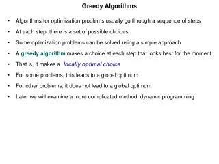
Overview • Like dynamic programming (DP), used to solve optimization problems. • Problems exhibit optimal substructure (like DP). • Problems also exhibit the greedy-choice property. • When we have a choice to make, make the one that looks best right now. • Make a locally optimal choicein hope of getting a globally optimal solution.
Greedy Strategy • The choice that seems best at the moment is the one we go with. • Prove that when there is a choice to make, one of the optimal choices is the greedy choice. Therefore, it’s always safe to make the greedy choice. • Show that all but one of the subproblems resulting from the greedy choice are empty.
Activity-selection Problem • Input: Set S of n activities, a1, a2, …, an. • si = start time of activity i. • fi = finish time of activity i. • Output: Subset A of maximum number of compatible activities. • Two activities are compatible, if their intervals don’t overlap. Example: Activities in each line are compatible.
Example: i 1 2 3 4 5 6 7 8 9 10 11 si1 3 0 5 3 5 6 8 8 2 12 fi4 5 6 7 8 9 10 11 12 13 14 {a3, a9, a11} consists of mutually compatible activities. But it is not a maximal set. {a1, a4, a8, a11} is a largest subset of mutually compatible activities. Another largest subset is {a2, a4, a9, a11}.
Optimal Substructure • Assume activities are sorted by finishing times. • f1 f2 … fn. • Suppose an optimal solution includes activity ak. • This generates two subproblems. • Selecting from a1, …, ak-1, activities compatible with one another, and that finish before ak starts (compatible with ak). • Selecting from ak+1, …, an, activities compatible with one another, and that start after ak finishes. • The solutions to the two subproblems must be optimal.
Recursive Solution • Let Sij = subset of activities in S that start after ai finishes and finish before aj starts. • Subproblems: Selecting maximum number of mutually compatible activities from Sij. • Let c[i, j] = size of maximum-size subset of mutually compatible activities in Sij. = f ì 0 if S Recursive Solution: ï ij = c [ i , j ] í + + ¹ f max{ c [ i , k ] c [ k , j ] 1 } if S ï ij î < < i k j
Greedy-choice Property • The problem also exhibits the greedy-choice property. • There is an optimal solution to the subproblem Sij, that includes the activity with the smallest finish time in set Sij. • Can be proved easily. • Hence, there is an optimal solution to S that includes a1. • Therefore, make this greedy choice without solving subproblems first and evaluating them. • Solve the subproblem that ensues as a result of making this greedy choice. • Combine the greedy choice and the solution to the subproblem.
Recursive Algorithm Recursive-Activity-Selector (s, f, i, j) • m i+1 • whilem < j and sm < fi • dom m+1 • ifm < j • thenreturn {am} Recursive-Activity-Selector(s, f, m, j) • else return Initial Call: Recursive-Activity-Selector (s, f, 0, n + 1) Complexity:(n) Straightforward to convert the algorithm to an iterative one. See the text.
Typical Steps • Cast the optimization problem as one in which we make a choice and are left with one subproblem to solve. • Prove that there’s always an optimal solution that makes the greedy choice, so that the greedy choice is always safe. • Show that greedy choice and optimal solution to subproblem optimal solution to the problem. • Make the greedy choice and solve top-down. • May have to preprocess input to put it into greedy order. • Example: Sorting activities by finish time.
Elements of Greedy Algorithms • Greedy-choice Property. • A globally optimal solution can be arrived at by making a locally optimal (greedy) choice. • Optimal Substructure.
Minimum Spanning Trees • Given: Connected, undirected, weighted graph, G • Find: Minimum - weight spanning tree, T • Example: 7 b c Acyclic subset of edges(E) that connects all vertices of G. 5 a 1 -3 3 11 d e f 0 2 b c 5 a 1 3 -3 weight of T: w(T) = d e f 0
Generic Algorithm • A - subset of some Minimum Spanning tree (MST). • “Grow” A by adding “safe” edges one by one. • Edge is “safe” if it can be added to A without destroying this invariant. A := ; while A not complete tree do find a safe edge (u, v); A := A {(u, v)} od
Definitions • Cut – A cut (S, V – S)of an undirected graph G = (V, E) is a partition of V. • A cut respects a set Aof edges if no edge in A crosses the cut. • An edge is a light edge crossing a cut if its weight is the minimum of any edge crossing the cut. cut that respects an edge set A = {(a, b), (b, c)} a light edge crossing cut (could be more than one) 5 7 a b c 1 -3 3 11 • cut partitions vertices into disjoint sets, S and V – S. d e f 0 2
Theorem 23.1 Theorem 23.1: Let (S, V - S) be any cut that respectsA, and let (u, v) be a light edge crossing (S, V - S). Then, (u, v) is safe for A. Proof: Let T be a MST that includes A. Case 1: (u, v) in T. We’re done. Case 2: (u, v) not in T. We have the following: edge in A (x, y) crosses cut. Let T´ = {T - {(x, y)}} {(u, v)}. Because (u, v) is light for cut, w(u, v) w(x, y). Thus, w(T´) = w(T) - w(x, y) + w(u, v) w(T). Hence, T´ is also a MST. So, (u, v) is safe for A. x cut y u shows edges in T v
Corollary In general, A will consist of several connected components (CC). Corollary: If (u, v) is a light edge connecting one CC in GA= (V, A) to another CC in GA, then (u, v) is safe for A.
Kruskal’s Algorithm • Starts with each vertex in its own component. • Repeatedly merges two components into one by choosing a light edge that connects them (i.e., a light edge crossing the cut between them). • Scans the set of edges in monotonically increasing order by weight. • Uses a disjoint-set data structure to determine whether an edge connects vertices in different components.
Prim’s Algorithm • Builds one tree. So A is always a tree. • Starts from an arbitrary “root” r. • At each step, adds a light edge crossing cut (VA, V - VA) to A. • VA= vertices that A is incident on. VA V - VA cut
Prim’s Algorithm 11 1 14 13 2 3 17 19 20 18 4 5 6 7 18 24 26 8 9 10 • Uses a priority queue Q to find a light edge quickly. • Each object in Q is a vertex in V - VA. implemented as a min-heap Min-heap as a binary tree.
Prim’s Algorithm • key(v) (key of v)is minimum weight of any edge (u, v), where u VA. • Then the vertex returned by Extract-Min is v such that there exists u VAand (u, v)is light edge crossing (VA, V - VA). • key(v) is if v is not adjacent to any vertex in VA. VA u1 V - VA w1 u2 w2 key(v) = min{w1, w2, w3} u3 v w3 v’ key(v’) = key(v’’) = v’’ cut
Prim’s Algorithm Q := V[G]; for each u Q do key[u] := od; key[r] := 0; [r] := NIL; whileQ do u := Extract-Min(Q); for each v Adj[u] do ifv Q w(u, v) < key[v] then [v] := u; key[v] := w(u, v) fi od od Complexity: Using binary heaps: O(E lgV). Initialization – O(V). Building initial queue – O(V). V Extract-Min’s – O(V lgV). E Decrease-Key’s – O(E lgV). Using min-heaps: O(E + VlgV). (see book) decrease-key operation Note:A = {([v], v) : v V - {r} - Q}.
Example of Prim’s Algorithm Not in tree 5 7 a/0 b/ c/ Q = a b c d e f 0 11 3 1 -3 d/ e/ f/ 0 2
Example of Prim’s Algorithm 5 7 a/0 b/5 c/ Q = b d c e f 5 11 3 1 -3 11 d/11 e/ f/ 0 2
Example of Prim’s Algorithm 5 7 a/0 b/5 c/7 Q = e c d f 3 7 11 11 3 1 -3 d/11 e/3 f/ 0 2
Example of Prim’s Algorithm 5 7 a/0 b/5 c/1 Q = d c f 0 1 2 11 3 1 -3 d/0 e/3 f/2 0 2
Example of Prim’s Algorithm 5 7 a/0 b/5 c/1 Q = c f 1 2 11 3 1 -3 d/11 e/3 f/2 0 2
Example of Prim’s Algorithm 5 7 a/0 b/5 c/1 Q = f -3 11 3 1 -3 d/11 e/3 f/-3 0 2
Example of Prim’s Algorithm 5 7 a/0 b/5 c/1 11 3 1 -3 d/11 e/3 f/-3 0 2 Q =
Example of Prim’s Algorithm 5 a/0 b/5 c/1 1 -3 3 d/0 e/3 f/-3 0