Greedy Algorithms
380 likes | 564 Views
Greedy Algorithms. Lecture 8 Prof. Dr. Aydın Öztürk. Introduction. A greedy algorithm always makes the choice that looks best at the moment. That is, it makes a locally optimal choice in the hope that this choice will lead to a globally optimal solution. An activity selection problem.

Greedy Algorithms
E N D
Presentation Transcript
Greedy Algorithms Lecture 8 Prof. Dr. Aydın Öztürk
Introduction • A greedy algorithmalways makes the choice that looks best at the moment. • That is, it makes a locally optimal choice in the hope that this choice will lead to a globally optimal solution.
An activity selection problem Suppose we have a set of n proposed activitiesthat wish to use a resource, such as a lecture hall, which can be used by only one activity at a time. Let si = start time for the activity ai fi=finish time for the activity ai where If selected, activity ai takes place during the half interval [si, fi).
An activity selection problem • aiand aj are competible if the intervals [si, fi) and [sj, fj) do not overlap. • The activity-selection problem: Select a maximum-size subset of mutually competible activities.
An example • Consider the following activities which are sorted in monotonically increasing order of finish time. • i 1 2 3 4 5 6 7 8 9 10 11 • si1 3 0 5 3 5 6 8 8 2 12 • fi4 5 6 7 8 9 10 11 12 13 14 • We shall solve this problem in several steps • Dynamic programming solution • Greedy solution • Recursive greedy solution
Dynamic programming solution to be the subset of activities in S that can start after activity ai finishes and finish before activity aj starts. Sijconsists of all activities that are compatible with aiand aj and are also compatible with all activities that finish no later than ai finishes and all activities that start no earlier than ajstarts. sj fi sk fk
Dynamic programming solution (cont.) Define Then And the ranges for iandj are given by Assume that the activities are sorted in finish time such that Also we claim that
Dynamic programming solution (cont.) Assuming that we have sorted the activities in monotonically increasing order of finish time, our space of subproblems is to select a maximum-size subset of mutually compatible activities from Sijfor knowing that all other Sij are empty.
Dynamic programming solution (cont.) • Consider some non-empty subproblem Sij , and suppose tha a solution to Sijincludes some activity ak, so that • Using activity ak, generates two subproblems: Sik and Skj . • Our solution to Sijis the union of the solutions to Sik and Skj along with the activity ak. • Thus, the # activities in our solution to Sijis the size ofsolution to Sik plusthe size ofsolution to Skj plus 1 for ak. Sik Skj ak fk sj sk fi
Dynamic programming solution (cont.) LetAijbe thesolution to Sij.Then, we have An optimal solution to the entire problem is a solution to S0,n+1.
A recursive solution The second step in developing a dynamic-programming solution is to recursively define the value of an optimal solution. Let c[ i, j] be the # activities in a maximum-size subset of mutuall compatible activities in Sij.Based on the definition ofAij we can write the following recurrence c[ i, j] = c[ i, k] + c[ k, j] +1 This recursive equation assumes that we know the value of k.
A recursive solution (cont.) There are j - i-1possible values ofk namelyk= i+1, ..., j-1. Thus, our full recursive defination of c[ i, j] becomes
It is straightforward to write a tabular, bottom-up dynamic-programming algorithm based on the above recurrence A bottom-up dynamic-programming solution
Converting a dynamic-programming solution to a greedy Theorem: Consider any nonempty subproblem Sij with the earliest finish time . Then 1. Activity amis used in some maximum-size subset of mutually competible activities of Sij . 2.The subproblemSim is empty, so that choosing am leaves the subproblem Smj as the only one that may be nonempty
Converting a dynamic-programming solution to a greedy (cont.) Important results of the Theorem: 1.In our dynamic-programming solution there were j-i-1 choices when solving Sij. Now, we have one choice and we need consider only one choice: the one with the earliest finish time in Sij. (The other subproblem is guaranteed to be empty) 2. We can solve each problem in a top-down fashion rather than the bottom-up manner typically used in dynamic programming.
Converting a dynamic-programming solution to a greedy (cont.) We note that there is a pattern to the subproblems that we solve: 1. Our original problem S = S0,n+1. 2. Suppose we chooseam1as the activity (in this case m1=1 ). 3. Our next sub-problem is and we choose as the activity in with the earliest finish time. 4. Our next sub problem is for some activity number m2. ...etc.
Recursive greedy algorithm RECURSIVE-ACTIVITY-SELECTOR(s, f, i, j) 1 m ← i+1 2 while m<j and sm<fi (Find the first activity) 3 do m ← m+1 • if m<j • then return {am}U RECURSIVE-ACTIVITY- SELECTOR(s, f, m, j) • else return Ø The initial call is RECURSIVE-ACTIVITY-SELECTOR(s, f, 0, n+1)
Recursive Greedy Algorithm RECURSIVE-ACTIVITY-SELECTOR(s, f, i, j) 1 m ← i+1 2 while m<j and sm<fi 3 do m ← m+1 if m<j then return{am}URECUR SIVE-ACTIVITY SELECTOR(s, f, m, j) else return Ø
Iterative greedy algorithm • We easily can convert our recursive procedure to an iterative one. • The following code is an iterative version of the procedure RECURSIVE-ACTIVITY-SELECTOR. • It collects selected activities into a set A and returns this set when it is done.
Iterative greedy algorithm GREEDY-ACTIVITY-SELECTOR(s, f) 1 n ← lengths[s] • A←{ a1} • i←1 • for m ← 2 ton • do if sm ≥ fi • then A←AU { am} • i←m • return A
Elements of greedy strategy • Determine the optimal substructure of the problem. • Develop a recursive solution • Prove that any stage of recursion, one of the optimal choices is greedy choice. • Show that all but one of the subproblems induced by having made the greedy choice are empty. • Develop a recursive algorithm that implements the greedy strategy. • Convert the recursive algorthm to an iterative algorithm.
Greedy choice property A globally optimal solution can be arrived at by making a locally optimal(greedy) choice. When we are considering which choice to make, we make the choice that looks best in the current problem, without considering results from subproblems
Greedy choice property (cont.) In dynamic programming, we make a choice at each step, but the choice usually depends on the solutions to subproblems. We typically solve dynamic-programming problems in a bottom-up manner. In a greedy algorithm, we make whatever choice seems best at the moment and then solve the subproblem arising after the choice is made. A greedy strategy usually progresses in a top-down fashion, making one greedy choice after another.
The 0-1 knapsack problem • A thief robbing a store finds n items; the ith item worths vi dollars and weighs wi pounds, where vi and wi are integers. • He wants to take as valuable a load as possible, but he can carry at most W pounds in his knapsack for some integer W. • Which item should he take?
The fractional knapsack problem • The set up is the same, but the thief can take fractions of items, rather than having to make a binary (0-1) choice for each item.
Huffman codes Huffman codes are widely used and very effective technique for compressingdata. We consider the data to be a sequence of charecters.
Huffman codes (cont.) A charecter coding problem: Fixed length code requires 300 000 bits to code Variable-length code requires 224 000 bits to code
Huffman codes (cont.) 100 100 1 0 1 0 55 a:45 a:45 14 86 0 1 0 0 1 58 28 25 30 14 0 0 1 0 1 0 1 0 1 1 a:45 b:13 d:16 d:16 e:9 f:5 c:12 b:13 14 d:16 c:12 0 1 f:5 e:9 Fixed-length code Variable-length code
Huffman codes (cont.) Prefix code: Codes in which no codeword is also a prefix of some other codeword. Encoding for binary code: Example:Variable-length prefix code. a b c Decoding for binary code: Example:Variable-length prefix code.
Constructing Huffman codes • Huffman’s algorithm assumes that Q is implemented as a binary min-heap. • Running time: • Line 2 : O(n) (uses BUILD-MIN-HEAP) • Line 3-8: O(n lg n) (the for loop is executed exactly n-1 times and each heap operation requires time O(lg n) )
Constructing Huffman codes: Example f:5 e:9 c:12 b:13 d:16 a:45 c:12 b:13 d:16 a:45 14 1 0 0 f:5 e:9 14 d:16 25 a:45 0 1 0 0 1 f:5 e:9 c:12 b:13
Constructing Huffman codes: Example a:45 25 30 0 1 0 1 c:12 b:13 d:16 14 0 1 f:5 e:9
Constructing Huffman codes: Example 55 a:45 1 0 30 25 0 0 1 1 d:16 14 c:12 b:13 0 1 f:5 e:9
Constructing Huffman codes: Example 100 1 0 55 a:45 1 0 30 25 0 1 0 1 d:16 14 c:12 b:13 1 0 f:5 e:9