Greedy Algorithms
Greedy Algorithms. Algorithms for optimization problems usually go through a sequence of steps At each step, there is a set of possible choices Some optimization problems can be solved using a simple approach A greedy algorithm makes a choice at each step that looks best for the moment

Greedy Algorithms
E N D
Presentation Transcript
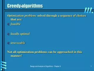
Greedy Algorithms • Algorithms for optimization problems usually go through a sequence of steps • At each step, there is a set of possible choices • Some optimization problems can be solved using a simple approach • A greedy algorithm makes a choice at each step that looks best for the moment • That is, it makes a locally optimal choice • For some problems, this leads to a global optimum • For other problems, it does not lead to a global optimum • Later we will examine a more complicated method: dynamic programming
Greedy Algorithm Design • We use the following sequence of steps • cast the optimization problem as one in which we make a choice and are then left with a single subproblem • prove that there is always an optimal solution to the original problem that makes the greedy choice (so the greedy choice is always safe) • demonstrate that after the greedy choice, the remaining sub-problem is such that if we combine the optimal solution to the sub-problem with the greedy choice that was made, the result is an optimal solution to the original problem.
Greedy Choice Property • Greedy Choice Property: A globally optimal solution can be obtained by making a sequence of locally optimal choices • In other words, at each step, we make the choice that looks best for the current problem, without considering results from sub-problems. • Thus greedy algorithms typically take a top-down approach • Dynamic programming takes a bottom-up approach
Greedy Algorithm for Coin Changing In the coin-changing problem, we are given a list of coin denominations and an amount A. The goal is to use as few of the coins as possible that total the amount A The greedy approach is to first use as many coins of the largest denomination as possible, which then reduces the amount to a value A1 less than the largest denomination. We then use the remaining coin denominations to give the remaining change using exactly the same strategy. Thus we would use as many coins of the second largest denomination, reducing the amount to be produced again. We continue until we reach the desired total. The algorithm is a greedy algorithm because the local strategy (for each step) is to generate as large an amount as possible that is less equal the current amount using as few coins as possible. It is obvious that this is done by giving as many coins of the largest possible denomination as possible.
Greedy Coin Changing • Given: - array denom of integers such that denom[1] > denom[2] > … > denom[n] = 1 • - integer A • Goal: make change for A using as few entries from denom as possible • greedy_coin_change(denom,A) { i = 1 • while (A > 0) { c = A/denom[i] • if ( c > 0 ) println(“use “ + c + “coins of denomination “ + denom[i] • A = A – c*denom[i] i = i+1 }}
Does the greedy coin changing algorithm work? Yes and no. It depends on the denominations If the denominations are 1, 6 and 10 the algorithm gives a non-optimal result for 12: 3 coins: one dime and two pennies. But we can use 2 6-cent pieces instead.
The algorithm does work for denominations 1, 5 and 10 We prove this by induction on A. Clearly you cannot do better for 1,2,3,4,5 and 10. If 5 < A < 10, the algorithm uses 1 five and (A-5) ones for a total of A-4 coins. But if you do not use a 5, you must use A ones. Now suppose A > 10 and the greedy algorithm works for all amounts less than A. Let k be the number of coins used in an optimal solution for A. Note that at most 4 coins of denomination 1 are used, because 5 ones can be replaced by one 5 for a net reduction of 4 coins. Also at most one 5 is used, because two 5’s could be replaced with a 10. Therefore the coins of denomination 1 and 5 can account for no more than 9 of the total of A. Since A > 9, at least one 10 coin is used. If you remove the 10 piece, the remaining coins must be optimal for amount A-10. By the inductive hypothesis, the change for A-10 was obtained by the greedy algorithm. But if we add in the 10 piece, this also arises from the greedy algorithm.
Greedy Example: Optimal Cell Tower Placement Scenario:Long, straight, quiet country road with houses scattered very sparsely along it. All residents are important people and are avid cell phone users. The range of your cell phone towers is 4 miles. Your goal: place cell phone towers along the road so that every residence is covered, using as few cell phone towers as possible. Model: A straight line with a left endpoint and right endpoint, a list x1, …, xn of locations for the individual houses (distance from the left endpoint) Solution: a sequence of real values c1, …, cm such that (1) for every i from 1 to n, there is a j from 1 to m so that |cj - xi| <= 4 (2) m is as small as possible subject to condition (1)
Cell Tower Placement Model: The road is modeled as a straight line with a left endpoint and a right endpoint. The house positions are given by their distance from the left endpoint, say h1, h2, …, hm. The output will be the cell tower distances from the left endpoint. Greedy approach: We want to place the first tower so that it covers the first house and as many more as possible; obvious choice: position h1 + 4. Having placed k of the towers, if we have not yet covered all houses, place the k+1st tower so that it covers the first uncovered house and as many beyond that as possible. Thus if hj is the first house (from left to right) not covered so far, put the next tower at position hj + 4. How would you prove that the above algorithm uses as few towers as possible?
Continuous Knapsack Problems • Input: a collection of objects such that each object has an associated weight and profit; and a total weight bound C. • Goal: choose an amount of each object between 0 and 1 so that the sum of the corresponding total profit is as large as possible • In this version of the problem, we do not have to take all of an object; we may subdivide it and take a part of the object. • If p is the proportion of the object taken, then the profit derived from the object is p times the profit value of the entire object • In the above, 0 p 1 • This version is known as the continuous(or fractional) knapsack problem • If we must either take all of the object (p = 1) or none of the object (p = 0), this version of the problem is called the 0/1-knapsack problem
Precise Statement – Continuous Knapsack Problem • Precise statement • Suppose we have n objects so that the ith object has weight wi and profit value pi • We are to find real values x1,x2,…,xn between 0 and 1 that maximize the total profit • subject to the constraint • Example(w1,p1) (w2,p2) (w3,p3) (w4,p4) (w5,p5) C(120,5) (150,5) (200,4) (150,8) (140,3) 600 If we take all of items 1, 2 and 4, 180 units of item 3 and none of item 5 we have values x1 = 1, x2 = 1, x3 = 180/200 = 0.9, x4 = 1 and x5 = 0. Then the total weight is 120 + 150 + 180 + 150 = 600 and the total profit is 1*5 + 1*5 + 0.9*4 + 1*8 = 21.6
Greedy Knapsack • In the homework, you will be asked to show that a greedy algorithm cannot be based on weight alone or profit alone • That is, if you always choose the minimum weight for the next guy to add (or the maximum weight), you will not necessarily maximize the total profit • Similarly, if you always choose the next item to be the one with the most profit regardless of weight, you will not always get an optimal solution • Instead, you should consider the profit/weight ratios, i.e., the amount of profit per unit weight • Thus the greedy algorithm specifies that you are to select the objects in non-increasing order of their price-to-weight ratio. You take all of the object if it will not exceed the capacity, otherwise you take as much as you can to reach the capacity.
Example • Recall our example:(w1,p1) (w2,p2) (w3,p3) (w4,p4) (w5,p5) C(120,5) (150,5) (200,4) (150,8) (140,3) 600 • The profit/weight ratios are p1/w1 = 5/120 = .0417; p2/w2 = 5/150 = .0333; p3/w3 = 4/200 = .0200; p4/w4 = 8/150 = .0533; p5/w5 = 3/140 = .0214; Thus the order of consideration is 4, 1, 2, 5, 3 We take all of items 4, 1, 2, and 5 for a total weight of 150 + 120 + 150 + 140 = 560 We now only have room for 40 units of weight, so we take 40/200 = 1/5 of object 3 The profit is thus 5 + 5 + 0.24 + 8 + 3 = 21.8
Greedy Knapsack Algorithm • continuous_knapsack(a,C) { // a is an array of items with weight, profit & id fields n = a.last for i = 1 to n ratio[i] = a[i].p/a[i].w sort(a,ratio) weight = 0 i = 1 while ( i n && weight < C ) { if (weight + a[i].w C) { println(“Select all of object “ + a[i].id) weight = weight + a[i].w } else { r = (C-weight)/a[i].w println(“Select “ + r +“ of object “ + a[i].id) weight = C } i = i+1 } }
Proof of Correctness • We can assume total weight exceeds capacity C • Let xi denote the portion of object i selected by the algorithm and let P be the total profit produced by the algorithm • Consider an arbitrary solution with portion amounts xi and total profit P. We will show that P P, which proves that the greedy solution is optimal • Since , we have • If k is the least index with xk < 1 and i < k, then xi = 1 and thus xi-xi 0. • Objects sorted in nondecreasing order of the ratio pi//wi so for all i < k • Thus if i < k, then • If i = k, then • If i > k, then xi = 0 and thus xi-xi 0. Also, by the sorted property, • Therefore, we again have
Proof of Correctness • On the previous slide we showed that for all k with 1 k n: • Recall that P is the greedy profit and P is the optimal profit • Thus the difference in the profits is • Thus P P and thus P = P , since P is the maximum possible profit
Homework Page 274: #2 Page 318: #2