Download
1 / 14
150 likes | 505 Views
Lecture 12: Phase diagrams. PHYS 430/603 material Laszlo Takacs UMBC Department of Physics. Phases and the phase rule. Phase: Uniform agglomeration of material - no boundaries inside Gibbs’ phase rule: f = n - p + 2

E N D
Lecture 12: Phase diagrams PHYS 430/603 material Laszlo Takacs UMBC Department of Physics
Phases and the phase rule Phase: Uniform agglomeration of material - no boundaries inside Gibbs’ phase rule: f = n - p + 2 f = degrees of freedom, i.e. number of freely selectable thermodynamic parameters. Typically temperature, pressure, concentrations. n = number of chemical components. p = number of phases in equilibrium When phases are in equilibrium, atoms of any component can be transferred between phases. Equilibrium requires equal chemical potentials, mathematically equations that reduce the number of freely selectable parameters.
The phase diagram of UF6 as a function of p and T n = 1, thus f = 3 - p
Pressure-temperature phase diagram of single component systems: sulfur and silicon dioxide.n = 1, thus f = 3 - p
The T-p phase diagram of FeUsually processes are carried out at atmospheric pressure, thus we will usually neglect the pressure dependence. Extreme high pressure does cause phase changes.
n = 2, thus f = 4 - p The phase diagram of a two-component system is usually shown for a fixed - ambient - pressure. The remaining variables are temperature and the concentration of either component. Notice: allotropic phases (Ti), solid solutions, compound phases, two-phase regions, transformations, etc.
The lever rule on the amount of each phase in a two-phase region Sample is 1 mole total, contains (1 - c) mole of component A c mole of component B We can also consider the sample as m mole ofphase with c plus m mole ofphase with c Total of component A in the sample 1 - c = m (1 - c) + m (1 - c) Total of component B in the sample c = mc + mc The sum of these two equations gives 1 = m + m as it should be. From the last two equations we get m = (c - c) / (c - c) m = (c - c) / (c - c) m / m = (c - c) / (c - c) c c c c = cB A B Notice that c is not the same as cA, even if phase is a solid solution based on A.
What determines the phase diagram? Equilibrium is given by the minimum of the Gibbs potential, G. If more than one phase are possible, the phase with the lowest G is the equilibrium state. G = H - TS At low temperature enthalpy dominates. Entropy becomes increasingly important at higher T. Ideal solution: Two chemically similar components G = H - T (Sv + SM) = GM - TSM Assume: • GM changes linearly from A to B. • Configurational entropy SM = -Nk [c ln c + (1-c) ln (1-c)] (same idea as with vacancies) The slope of SM goes to */- ∞ when c --> 0 or 1
G(T,c) of an ideal solution GM is a simple weighted average of the Gibbs potential of the components and ∆Sm is the configurational entropy. Notice that the entropy term becomes more important with increasing temperature, increasing the curvature of the G(c) curve.
Comparing G for the ideal solution and the similar G for the liquid phase allows the construction of a hypothetical phase diagram. Notice that S is lower for low, L is lower for high temperature. Notice the changing curvature. In intermediate states, neither L nor S gives the smallest possible G. The state is a mixture of the two; common tangent gives the concentrations, the lever rule gives the relative amounts.
Why the common tangent? For an average concentration of c, we have x fraction with c1 and (1 - x) with c2. c = x c1 + (1 - x) c2, thus x = (c2 - c) / (c2 - c1); 1 - x = (c - c1) / (c2 - c1) The Gibbs potential for the mixture G = G1 x + G2 (1 - x) = G1 (c2 - c) / (c2 - c1) + G2 (c - c1) / (c2 - c1) This is a linear equation that describes a straight line between the end points. We get the lowest G when finding the lowest straight line still having end points on the G(c) curve - that is the common tangent. G1 G2 c1 c c2
Regular solutions Beside mixing entropy, differences in nearest neighbor bond energy provide a variation of the enthalpy term: HAA, HBB, HAB. Suppose N atoms (A and B together), z nearest neighbors, c is concentration of B. NAA = 1/2 * N (1-c) * z(1-c) = 1/2 * (total A) * (mean A neighbor) NBB = 1/2 * N c * z c NAB = N z c (1-c) Hm = NAAHAA + NBBHBB + NABHAB = 1/2 Nz [(1-c)HAA + cHBB + 2c(1-c)H0] where H0 = HAB - 1/2(HAA + HBB) The last term in Hm has a maximum for H0 > 0, competes with the minimum caused by configurational entropy. The slope of entropy is +/- ∞ at the borders, the slope of Hm is finite. Can result in limited solubility. G = Hm - TSm
Gibbs’ free energy for a regular solution: • H0 < 0 makes Gm sharply peaked - ordering, compound formation • H0 > 0 can result in two minima. For c1 < c < c2, the lowest energy state is a mixture - phase separation, limited mutual solubility. If HAA = HBB and c << 1, the solubility limit from dG/dc = 0 is c1 = exp(-zH0/kT)