Download
1 / 13
130 likes | 274 Views
Vibrations in linear 1-dof systems; III. damped systems (last updated 2011-08-28). Aim.

E N D
Vibrations in linear 1-dof systems;III. damped systems (last updated 2011-08-28)
Aim The aim of this presentation is to give a short review of basic vibration analysis of dampedlinear 1 degree-of-freedom (1-dof) systems.For a more comprehensive treatment of the subject, see any book on vibration analysis.
A simple example Let us study the effect of linear damping by considering the following simpleexample. where Fd is a damping force, having any kind of physical origin. By making afree body diagram of the (point) mass, we get where the coordinate x describes the position of the mass (equal to thedeflection of the rod), and where the force S represents the interactionbetween the rod and the point mass. Elementary solid mechanics now gives
A simple example; cont. By assuming a linear damping we get or Thus, the lateral motion of the mass as a function of time is governed by alinear 2'nd order ordinary differential equation with constant coefficients! The solution is given by the sum of the homogeneous solution and theparticular solution, , where the former corresponds to theself vibration of the mass caused by the initial conditions (placement andvelocity), while the latter is caused by the applied force.
A simple example; cont. Homogeneous solution For the homogeneous solution we have • Depending on the size of ζ we may now get • two different imaginary roots (for ζ <1); case of weak damping • two equal real roots (for ζ =1); case of critical damping • two different real roots (for ζ >1); case of strong damping • The reason for the labels weak, critical and strong will be motivated below.
A simple example; cont. Homogeneous solution; weak damping (ζ <1) As can be seen, the homogeneous solution decays as a periodic function withdecreasing amplitude.
A simple example; cont. Homogeneous solution; critical damping (ζ =1) As can be seen, the homogeneous solution decays as a non-periodic/aperiodicfunction. For this case we may define the critical damping parameter ccrit
A simple example; cont. Homogeneous solution; strong damping (ζ >1) As can be seen, the homogeneous solution again decays as an aperiodicfunction. A final comment is that the label "critical damping" by no way means that it iscritical in some way– it only indicates that it is the lowest value of ζ(and thus for c) for which an aperiodic motion can exist.
A simple example; cont. Particular solution For the particular solution, valid at stationary conditions, we have
A simple example; cont. Particular solution; cont.
A simple example; cont. Particular solution; cont.
A simple example; cont. Particular solution; cont.
A simple example; cont. • Particular solution; cont. • For the damped case we note that • there is no resonance frequency in a strict sense, since the damping will make the stationary vibration amplitude finite for all applied frequencies • the dynamic impact factor and thus the vibration amplitude may however become very large if the damping is small