Hash Tables
530 likes | 801 Views
Hash Tables. Tonga Institute of Higher Education. Introduction. Hash tables are another data structure that can hold data. Advantages Hash tables are very good at insertion and searching No matter how much data you have, insertions, searches and sometimes deletions are close to O(1) time

Hash Tables
E N D
Presentation Transcript
Hash Tables Tonga Institute of Higher Education
Introduction • Hash tables are another data structure that can hold data. • Advantages • Hash tables are very good at insertion and searching • No matter how much data you have, insertions, searches and sometimes deletions are close to O(1) time • Disadvantages • When hash tables become too full, performance degrades very quickly • Hash tables are based on arrays, and arrays are difficult to expand • You cannot move from data item to data item in any kind of order • Therefore, you must make sure you have an accurate idea of how much data you will store. • Also, you must not need to visit the data in any order.
Arrays are Useful • Arrays are useful in certain situations • If you have a system to keep track of your employees, you can use an array • Each employee record occupies one cell of the array • The array number could be the Employee ID number • So looking up employee data is easy if you know the Employee ID number
Array Shortcomings • However, when arrays get very large, they take a long time to search through them. • Unordered arrays take a long time to search for items • Search: O(N) time • Ordered arrays take a long time when new data items are added • Search: O(log N) time • Insert: O(N) time • Let’s say we are asked to make a English dictionary and put it on the web • Stores 100,000 English words • Each word needs to be quickly accessible • Sometimes, new words are added • A hash table is a good choice for a dictionary • Search: O(1) time • Insert: O(1) time
Hash Tables • Hash tables use an array behind the scenes • The index of each cell is calculated using a formula • Hashing – Converting a value from one set to another • Hash Value or Hash - A number generated from another value like a string of text • The hash is substantially smaller than the text itself, and is generated by a formula in such a way that it is extremely unlikely that some other text will produce the same hash value.
Demonstration Hash Applet
Hashing – Addition Formula • Simple formula where we add digits • A = 1, B = 2, C = 3, …, S = 19, T = 20, …, Z = 26 • CATS = 3 + 1 + 20 + 19 = 43 • So the index of CATS would be 43 • But this is not a good choice • If we restrict ourselves to 10 letter words, the last word would potentially be: • zzzzzzzzzz = 26 + 26 + 26 + 26 + 26 + 26 + 26 + 26 + 26 + 26 = 260 • So the range of indexes would be from 1 to 260. (a to zzzzzzzzzz) • But we know that there are more than 260 words • This is because many words add up to 43: bails, was, tin, tick, give, tend, moan,
Hashing – Multiplication by Powers Formula - 1 • With normal numbers • Each digit can be from 0 to 9. (10 different values) • Each digit position represents a value 10 times as big as the digit position to the right • 7654 • 7 * 1000 + 6 * 100 + 5 * 10 + 5 * 1 • 7 * 103 + 6 * 102 + 5 * 101 + 5 * 100 • 7654 • This guarantees that every possible number has a unique numerical value
Hashing – Multiplication by Powers Formula - 2 • With letters • We can apply the same idea to guarantee that each letter sequence has a unique numerical value • Each character can be from a to z. (26 different values) • Each character position represents a value 26 times as big as the character position to the right • A = 1, B = 2, C = 3, …, S = 19, T = 20, …, Z = 26 • CATS • (3 * 263) + (1 * 262) + (20 * 261) + (19 * 260) • (3 * 17576) + (1 * 676) + (20 * 26) + (19 * 1) • 53943 • This guarantees that every possible letter combination has a unique numerical value
Hashing – Multiplication by Powers Formula - 3 • But even this is not a good choice • If we restrict ourselves to 10 letter words, the last word would potentially be: • zzzzzzzzzz • 26 * 269 + 26 * 268 + 26 * 267 + 26 * 266 + 26 * 265 + 26 * 264 + 26 * 263 + 26 * 262 + 26 * 261 + 26 * 260 • This number is very big: 269 alone is 5.4295E+12! • This value is too big for an array to store in memory! • This is because every single letter combination computes into a unique index. Not every letter combination is a word! (Example: afwe, oijaw, awioa)
Hashing – Modulo Operator • The Multiplication by Powers formula • Gives us a unique number for every letter combination up to 10 letters long • Has too many values • We need a way to compress the huge range of numbers into a range that that is smaller • Our English dictionary will have 100,000 values • We can use the Modulo operator (%) to accomplish this
Modulo Operator • The Modulo operator gives us the remainder when one number is divided by another • Example 1 • 13 % 10 = 3 • 13 divided by 10 results in a remainder of 3 • Example 2 • 26 % 5 = 1 • 26 divided by 5 results in a remainder of 1 • So what is the remainder for these? • 55 % 6 • 73 % 73 • 13 % 8
Hashing with the Modulo Operator • Using the Modulo Operator, we can make every value in a large range of values map to a value in a small range of values • In the huge range, each number represents a potential word, but few of the numbers represent real words • In the small range, we can make it so half of cells are full SizeOfSmallArray = numberOfPlannedDataItems * 2 • Then, we use a hash function to map a value from the huge range to the small range IndexInSmallArray = KeyInLargeArray % SizeOfSmallArray This formula is only true for open addressing
Collisions • We pay a price for squeezing a large range into a small range • Sometimes, two values from the large range will equal the same value in the small range • We hope that not too many words will hash to the same index • Collision - When we have 2 large range values that hash to the same small range value Both words occupy the same location
Handling Collisions • There are 2 main ways to handle collisions • Open Addressing – When a data item can’t be placed at a particular index, another location in the array is used • Linear probing • Quadratic probing • Double hashing • Separate Chaining – When more than 1 data item needs to be placed at a particular index, linked lists are used
Open Addressing - Linear Probing • In linear probing, when we try to insert and have a collision, we search sequentially for an empty cell • Example: If 53 is occupied we try 54 then 55 and so on until we find an empty cell • The index is incremented until we find an empty cell • At the end of the list, loop around and continue at the beginning of the list • This is called linear probing because it steps sequentially along the line of cells To simplify our examples we will use number keys
Demonstration Hash Applet: Insert
Code View Hash Insert
Open Addressing - Linear Probing Searching The original key is 472 Using a hash function results in an index of 52 • When searching for a data item we follow these steps • Use a hash function on the key to get an index for the small range • Check the item located at the index to see if it has the same key • Keep looking until we find an item with the same key or we find an empty cell The original key is 135 Using a hash function results in an index of 53
Demonstration Hash Applet: Searching
Code View Hash Search
Open Addressing - Linear Probing Deleting • When we delete an item, we can’t clear the cell • This is because the find routine quits when it finds an empty cell • Therefore, we mark the cell as being deleted with a -1 • The insert code should then be able to insert items in an empty cell or a cell with a deleted value If we cleared 413, how would 532 and 472 be found?
Demonstration Hash Applet: Delete
Code View Hash Delete
Primary Clustering • When using linear probing, filled cells are not evenly distributed in our array • Sometimes, there’s a sequence of empty cells • Sometimes, there’s a sequence of filled cells • Cluster - A sequence of filled cells • Clustering can result in very long probe lengths. Therefore, getting to cells at the end of a sequence is slow • The bigger the cluster, the faster it will grow • Linear probing is not used very often because it suffers from too much primary clustering
Avoiding Primary Clustering • If a hash table has many large clusters, the array may be too small • Increasing the size of the array will help prevent further clustering • This will require • The creation of a new and larger hash table • The copying of values from the old hash table to the new hash table • Do not copy the values from the old hash table to cells that are next to each other. This will create 1 huge cluster. • Instead, use the insert() method for the new hash table • This processing is called rehashing
Open Addressing - Quadratic Probing • Quadratic probing eliminates primary clustering • In linear probing, when we try to insert and have a collision, we search sequentially for an empty cell • 1st index = x • 2nd index = x + 1 • 3rd index = x + 2 • 4th index = x + 3 • In quadratic probing, when we try to insert and have a collision, we search for an empty cell using this formula • 1st index = x • 2nd index = x + 12 = x + 1 • 3rd index = x + 22 = x + 4 • 4th index = x + 32 = x + 9 • 5th index = x + 42 = x + 16 • At the end of the list, loop around and continue at the beginning of the list • The index is increased until we find an empty cell • This is called quadratic probing because it steps sequentially along the line of cells using squares of values
Secondary Clustering • Quadratic probing eliminates primary clustering • However, it’s performance can still suffer if many items use the same key • For example, if 184, 352, 973, 1352 and 1705 all hash to the same index, a probe for 1705 takes a long time • This phenomenon is called secondary clustering • Secondary clustering is not a serious problem • Quadratic hash tables are not used very often because it can suffer from secondary clustering
Open Addressing - Double Hashing • Double Hashing is better than Quadratic Probing • Double hashing eliminates secondary clustering • Each step is different • The double hashing formula can be calculated faster than the quadratic probing formula • The number of steps taken depends on the key instead of the same sequence being used over and over again (1, 2, 4, 9, 25…) • This is done by hashing the key a second time, using a different hash function, and using the result as a step size • The secondary hash function must follow these rules • It must not be the same as the primary hash function • It must never output a 0 because otherwise there would never be a step and the algorithm would be in an never-ending loop • Experts have found that the following formula works well stepSize = constant – (KeyInBigArray % constant) • At the end of the list, loop around and continue at the beginning of the list If the constant is 5, the step sizes will range from 1 to 5!
Demonstration HashDouble Applet
Code View HashDouble
Open Addressing Hash Array Size • Double hashing requires that the array size be a prime number • A prime number is a number that cannot be evenly divided by another number • 2, 3, 5, 7, 11, 13, 17, 19, 23, etc. • A prime number is required to avoid a situation like this: • An array size is 15 (indices from 0 to 14) • A key hashes to 0 with a step size of 5 • This results in a never-ending step sequence: 0, 5, 10, 0, 5, 10… • The program would crash • Using a prime number make it impossible for any number to divide evenly, so every remaining cell will be checked
Handling Collisions • There are 2 main ways to handle collisions • Open Addressing – When a data item can’t be placed at a particular index, another location in the array is used • Linear probing • Quadratic probing • Double hashing • Separate Chaining – When more than 1 data item needs to be placed at a particular index, linked lists are used
Separate Chaining • Separate chaining – When more than 1 data item needs to be placed at a particular index, linked lists are used • The idea of separate chaining is easier to understand for many people • However, it requires more code to implement the linked lists
Demonstration HashChain Applet
Code View HashChain
Separate Chaining Hash Small Array Size • We know: smallArrayIndex = largeKey % smallArraySize • The small array size must be a prime number
Load Factors • Load Factor – The ratio of the number of items in an array to the array size loadFactor = numberOfItems / arraySize • In open addressing, performance degrades badly when a load factor is above .5 • In separate chaining hash tables, it is ok for load factors to be higher than 1 • Finding the initial cell takes O(1) time and searching through the list requires time proportional to the length of the list which is O(N) • Thus, separate chaining hash tables are preferred over open addressing hash tables. Especially when you don’t know in advance how much data will be in the hash table
Hash Functions • What makes a good hash function? • It must be quick to compute • Addition is faster than multiplications, divisions and exponents • A hash table with many multiplications, divisions and exponents is bad • It must also produce values that are evenly distributed across the possible range of values • Random distributions are even over the long run
Random and Non-Random Keys • Random Keys • If our keys are random, our initial formula works well smallArrayIndex = largeKey % smallArraySize • Non-Random Keys • Often, we do not use random keys • For example, some companies may have an id like this • 033-400-03-94-05-5-535 • Digits 0-2: Supplier number (1 to 999) (Currently up to 70) • Digits 3-5: Category code (100, 150, 200, 250, up to 850) • Digits 6-7: Month of introduction (1 to 12) • Digits 8-9: Year of introduction (00 to 99) • Digits 10-11: Serial Number (1 to 99) • Digit 12: Toxic risk flag (0 or 1) • Digit 13-15: Checksum (Sum of other fields, modulo 100) • In this case, many numbers may not be used • How can we ensure that the hash function results will be truly random?
Non Random Keys • Don’t use non-data • Key fields should be reduced until every bit counts. • For example, the category code should run from 0 to 15 • Also, the checksum is redundant so remove it • Use all the data • Every part of the key that has real data should contribute to the key used in the hash function • Always use a prime number for the modulo base • If keys share a divisor with the array size, they may hash to the same location, causing clustering • A prime number eliminates the possibility of this occurring
Folding - 1 • Another good hash function involves folding • This means you divide the key into groups of digits and add the groups together. • This ensures that all the digits influence the hash value • For example, each US citizen is identified by a Social Security number • 975-27-8237 • 123-45-6789 • First, pick the size you want your array to be • Array size = 1000 smallArrayIndex = largeKey % smallArraySize • Therefore, use 1000 as the value used by the modulo • Therefore, the largeKey must be big enough to give a big range of values when the modulo of 1000 is used on it • When folding, we break the number up like this • 12 + 34 + 56 + 78 + 9 = 189 • But this is not good because using a modulo of 1000 with this number will give us a range of 1 – 189 • 123 + 456 + 789 = 1368 • This is better because using a modulo of 1000 with this number will give us a range of 1 - 999 • Then, we get the remainder of a modulo operation to get our small array index • 1368 % 1000 = 368 • The size of the array changes the digit group size • Also, in real life, the smallArraySize would be a prime number. 1000 is used to make the example clear
Folding - 2 • If we want our array size to be 100 • When folding, we break the number up like this • 12 + 34 + 56 + 78 + 9 = 189 • This is ok because using a modulo of 100 with this number will give us a range of 1 – 99 • The size of the array changes the digit group size
Hashing Efficiency • If no collisions occur, insertion and searching in hash tables are O(1) time • This only involves a call to the hash function and a single array reference • If a collision occurs, access times are • The time described above O(1) + probe length • Probe length – How many times we need to search for a data item after the collision occurs • As the load factor increases, the probe length increases
Open Addressing Linear Probing Performance • The loss of efficiency with high load factors is more serious for open addressing than separate chaining • Unsuccessful searches generally take longer • During a successful probe sequence, the algorithm can stop as soon as it finds the desired item, which is, on average, halfway through the probe sequence • During an unsuccessful probe sequence, the algorithm must search the entire sequence before it’s sure the item is not found
Open Addressing Quadratic Probing and Double Hashing Performance • Quadratic probing and double hashing performance is the same • The performance is better than linear probing • Higher load factors can be tolerated for quadratic probing and double hashing than linear probing
Separate Chaining Performance • A load factor of 1.0 is fairly common • Smaller load factors do not improve performance significantly • Speed for all operations increases linearly with load factor
Open Addressing vs. Separate Chaining • Generally, if you use open addressing, use double hashing as it is better than linear probing and quadratic probing • If you don’t know how many items will be inserted into a hash table, then use separate chaining. • Increasing the load factor causes major performance problems with open addressing • Increasing the load factor degrades performance linearly with separate chaining • When in doubt, use separate chaining • It is more work at first • But the reward is that adding more data won’t degrade performance too badly
Using HashTables in Java 1 • Each string has a hashCode method. Some hash codes are the same!
Using HashTables in Java 2 • The hashcode for a String object is computed as: s[0]*31^(n-1)+s[1]*31^(n-2)+...+s[n-1] • Where s[i] is the ith character of a string of length n • The hash value of an empty string is defined as zero