Download
1 / 29
290 likes | 331 Views
Learn about hash functions, collision handling, and hash code maps. Explore chaining, linear probing, double hashing, and more. Understand perfect hash functions and example applications.

E N D
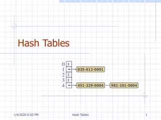
Hash Tables 0 1 025-612-0001 2 3 4 451-229-0004 981-101-0004 Hash Tables
Outline and Reading • Hash functions and hash tables (§8.3) • Hash function details • Hash code map (§8.3.3) • Compression map (§8.3.4) • Collision handling (§8.3.5) • Chaining • Linear probing • Double hashing Hash Tables
Hashing: • A method for directly referencing items in a dictionary by doing arithmetic transformations on keys into dictionary addresses. • A hush function is perfect if there is no key collision, that is, two keys hash to the same hash value. Hash Tables
An Example: • suppose: MagicNumber = 15 • inth(String s) { return ((s[0] + s[1])% MagicNumber); } • suppose: planet solarSystem[MagicNumber]; class planet { String name; int numMoons; double sunDistance; …. } Hash Tables
Suppose: solarSystem[h(“Mercury”)] = new planet(“Mercury”, 0, 36.0); solarSystem[h(“Venus”)] = new planet(“Venus”, 0, 67.27); solarSystem[h(“Earth”)] = new planet(“Earth”, 1, 93.0); solarSystem[h(“Mars”)] = new planet(“Mars”, 2, 141.71); solarSystem[h(“Jupiter”)] = new planet(“Jupiter”, 16, 483.88); solarSystem[h(“Saturn”)] = new planet(“Saturn”, 12, 887.14); solarSystem[h(“Uranus”)] = new planet(“Uranus”, 5, 1783.98); solarSystem[h(“Neptune”)] = new planet(“Neptune”, 2, 2795); solarSystem[h(“Pluto”)] = new planet(“Pluto”, 1, 3675); • Where are they located Hash Tables
“Ju” in ASCII are 74 and 117, 74 + 117 = 191; 191 % 15 = 11; h(“Mercury”) = 13 h(“Venus”) = 7 h(“Earth”) = 1 h(“Mars”) = 9 h(“Jupiter”) = 11 h(“Saturn”) = 0 h(“Uranus”) = 4 h(“Neptune”) = 14 h(“Pluto”) = 8 Thus, our search function is simply: planet search(String s){ return solarSystem[h(s)]; } Hash Tables
A hash functionh maps keys of a given type to integers in a fixed interval [0, N- 1] Example:h(x) =x mod Nis a hash function for integer keys The integer h(x) is called the hash value of key x The goal of a hash function is to uniformly disperse keys in the range [0, N- 1] A hash table for a given key type consists of Hash function h Array (called table) of size N When implementing a dictionary with a hash table, the goal is to store item (k, o) at index i=h(k) A collision occurs when two keys in the dictionary have the same hash value Collision handing schemes: Chaining: colliding items are stored in a sequence Open addressing: the colliding item is placed in a different cell of the table Hash Functions and Hash Tables Hash Tables
Example • We design a hash table for a dictionary storing items (SSN, Name), where SSN (social security number) is a nine-digit positive integer • Our hash table uses an array of sizeN= 10,000 and the hash functionh(x) = last four digits of x • We use chaining to handle collisions 0 1 025-612-0001 2 3 4 451-229-0004 981-101-0004 … 9997 9998 200-751-9998 9999 Hash Tables
A hash function is usually specified as the composition of two functions: Hash code map:h1:keysintegers Compression map:h2: integers [0, N- 1] The hash code map is applied first, and the compression map is applied next on the result, i.e., h(x) = h2(h1(x)) The goal of the hash function is to “disperse” the keys in an apparently random way Hash Functions Hash Tables
Memory address: We reinterpret the memory address of the key object as an integer (default hash code of all Java objects) Good in general, except for numeric and string keys Integer cast: We reinterpret the bits of the key as an integer Suitable for keys of length less than or equal to the number of bits of the integer type (e.g., byte, short, int and float in Java) Component sum: We partition the bits of the key into components of fixed length (e.g., 16 or 32 bits) and we sum the components (ignoring overflows) Suitable for numeric keys of fixed length greater than or equal to the number of bits of the integer type (e.g., long and double in Java) Hash Code Maps Hash Tables
Polynomial accumulation: We partition the bits of the key into a sequence of components of fixed length (e.g., 8, 16 or 32 bits)a0 a1 … an-1 We evaluate the polynomial p(z)= a0+a1 z+a2 z2+ … … +an-1zn-1 at a fixed value z, ignoring overflows Especially suitable for strings (e.g., the choice z =33gives at most 6 collisions on a set of 50,000 English words) Polynomial p(z) can be evaluated in O(n) time using Horner’s rule: The following polynomials are successively computed, each from the previous one in O(1) time p0(z)= an-1 pi(z)= an-i-1 +zpi-1(z) (i =1, 2, …, n -1) We have p(z) = pn-1(z) Hash Code Maps (cont.) Hash Tables
Division: h2 (y) = y mod N The size N of the hash table is usually chosen to be a prime The reason has to do with number theory and is beyond the scope of this course Multiply, Add and Divide (MAD): h2 (y) =(ay + b)mod N a and b are nonnegative integers such thata mod N 0 Otherwise, every integer would map to the same value b Compression Maps Hash Tables
Linear probing handles collisions by placing the colliding item in the next (circularly) available table cell Each table cell inspected is referred to as a “probe” Colliding items lump together, causing future collisions to cause a longer sequence of probes Example: h(x) = x mod13 Insert keys 18, 41, 22, 44, 59, 32, 31, 73, in this order Linear Probing 0 1 2 3 4 5 6 7 8 9 10 11 12 41 18 44 59 32 22 31 73 0 1 2 3 4 5 6 7 8 9 10 11 12 Hash Tables
Consider a hash table A that uses linear probing findElement(k) We start at cell h(k) We probe consecutive locations until one of the following occurs An item with key k is found, or An empty cell is found, or N cells have been unsuccessfully probed Search with Linear Probing AlgorithmfindElement(k) i h(k) p0 repeat c A[i] if c= returnNO_SUCH_KEY else if c.key () =k returnc.element() else i(i+1)mod N p p+1 untilp=N returnNO_SUCH_KEY Hash Tables
To handle insertions and deletions, we introduce a special object, called AVAILABLE, which replaces deleted elements removeElement(k) We search for an item with key k If such an item (k, o) is found, we replace it with the special item AVAILABLE and we return element o Else, we return NO_SUCH_KEY insert Item(k, o) We throw an exception if the table is full We start at cell h(k) We probe consecutive cells until one of the following occurs A cell i is found that is either empty or stores AVAILABLE, or N cells have been unsuccessfully probed We store item (k, o) in cell i Updates with Linear Probing Hash Tables
Double hashing uses a secondary hash function d(k) and handles collisions by placing an item in the first available cell of the series (i+jd(k)) mod Nfor j= 0, 1, … , N - 1 The secondary hash function d(k) cannot have zero values The table size N must be a prime to allow probing of all the cells Common choice of compression map for the secondary hash function: d2(k) =q-k mod q where q<N q is a prime The possible values for d2(k) are1, 2, … , q Double Hashing Hash Tables
Example of Double Hashing • Consider a hash table storing integer keys that handles collision with double hashing • N= 13 • h(k) = k mod13 • d(k) =7 - k mod7 • Insert keys 18, 41, 22, 44, 59, 32, 31, 73, in this order 0 1 2 3 4 5 6 7 8 9 10 11 12 31 41 18 32 59 73 22 44 0 1 2 3 4 5 6 7 8 9 10 11 12 Hash Tables
Performance: • Let N be the number of slots of a hash table, n be the number of items in the table, we define load factor as: = n/N • If the hash function randomly distributes keys through the table, then the expected length of a successful search path is: lengthsucc = ½(1 + 1/(1- )) Hash Tables
Performance: • The expected length of an unsuccessful search is approximately: lengthunsucc = ½( 1 + 1/(1 - )2) Hash Tables
Problems with Probing: • The size of the hash table must be fixed in advance. • The search costs increase dramatically as the table becomes nearly full. • Need a special object, called AVAILABLE, to implement “delete” operation. Hash Tables
Collision resolution using Linked Lists: • Dynamically allocate space. • Easy to insert/delete an item • Need a link for each node in the hash table. Hash Tables
Performance: • Let N be the size of the hash table, n the number of items in the table’s linked lists, if all input sequences are equally likely and the hash function randomly distributes keys over the table, the expected length of a linked list is n/N. lengthsucc = ½(n/N) lengthunsucc = n/N Hash Tables
In the worst case, searches, insertions and removals on a hash table take O(n) time The worst case occurs when all the keys inserted into the dictionary collide The load factor a=n/N affects the performance of a hash table Assuming that the hash values are like random numbers, it can be shown that the expected number of probes for an insertion with open addressing is1/ (1 -a) The expected running time of all the dictionary ADT operations in a hash table is O(1) In practice, hashing is very fast provided the load factor is not close to 100% Applications of hash tables: small databases compilers browser caches Conclusion: Hash Tables
a 3 Locators g e 1 4 Hash Tables
Outline and Reading • Locators (§8.7) • Locator-based methods • Implementation • Positions vs. Locators Hash Tables
A locators identifies and tracks a (key, element) item within a data structure A locator sticks with a specific item, even if that element changes its position in the data structure Intuitive notion: claim check reservation number Methods of the locator ADT: key(): returns the key of the item associated with the locator element(): returns the element of the item associated with the locator Application example: Orders to purchase and sell a given stock are stored in two priority queues (sell orders and buy orders) the key of an order is the price the element is the number of shares When an order is placed, a locator to it is returned Given a locator, an order can be canceled or modified Locators Hash Tables
Locator-based priority queue methods: insert(k, o): inserts the item (k, o) and returns a locator for it min(): returns the locator of an item with smallest key remove(l): remove the item with locator l replaceKey(l, k): replaces the key of the item with locator l replaceElement(l, o): replaces with o the element of the item with locator l locators(): returns an iterator over the locators of the items in the priority queue Locator-based dictionary methods: insert(k, o): inserts the item (k, o) and returns its locator find(k): if the dictionary contains an item with key k, returns its locator, else return the special locator NO_SUCH_KEY remove(l): removes the item with locator l and returns its element locators(), replaceKey(l, k), replaceElement(l, o) Locator-based Methods Hash Tables
Implementation d 6 • The locator is an object storing • key • element • position (or rank) of the item in the underlying structure • In turn, the position (or array cell) stores the locator • Example: • binary search tree with locators a b 3 9 g e c 1 4 8 Hash Tables
Position represents a “place” in a data structure related to other positions in the data structure (e.g., previous/next or parent/child) implemented as a node or an array cell Position-based ADTs (e.g., sequence and tree) are fundamental data storage schemes Locator identifies and tracks a (key, element) item unrelated to other locators in the data structure implemented as an object storing the item and its position in the underlying structure Key-based ADTs (e.g., priority queue and dictionary) can be augmented with locator-based methods Positions vs. Locators Hash Tables