Download

1 / 60
610 likes | 775 Views
Hash Tables. Saurav Karmakar. Motivation. What are the dictionary operations? (1) Insert (2) Delete (3) Search (most of the time, we will be focusing on search). Objective. Searching takes Θ (n) time in the worst case (when the data is unorganized).

E N D
Hash Tables Saurav Karmakar
Motivation • What are the dictionary operations? (1) Insert (2) Delete (3) Search (most of the time, we will be focusing on search)
Objective • Searching takes Θ(n) time in the worst case (when the data is unorganized). • Even using binary search it takes Θ(log n) time when the data are sorted. • Our Objective? O(1) time on average using hashing, under a reasonable assumption.
Definitions • A hash table is a generalization of an array (direct addressing is allowed), so let’s first talk about direct-address table. • Universe of keys U={0,1,2,…,m-1}, no two elements have the same key. • To represent a dynamic set, we use an array, or direct address table T[0..m-1], in which each position (slot) corresponds to the key in the universe.
Definitions • To represent a dynamic set, we use an array, or direct address table T[0..m-1], in which each position (slot) corresponds to a key in the universe. T satellite data 0 / key 1 / 2 2 U (universe of keys) 3 3 • 1 • 0 / 4 • 2 • 9 • 3 K (actual keys) • 4 5 5 • 8 6 / • 5 7 / 8 8 9 /
With a direct address table T[0..m-1], how do we search an element x with key k? Direct-Address-Search(T,k): return T[k] T satellite data 0 / key 1 / 2 2 U (universe of keys) 3 3 • 1 • 0 / 4 • 2 • 9 • 3 K (actual keys) • 4 5 5 • 8 6 / • 5 7 / 8 8 9 /
With a direct address table T[0..m-1], how do we search/insert/delete an element x with key k? Direct-Address-Search(T,k): return T[k] Direct-Address-Insert(T,x): T[key[x]] ← x Direct-Address-Delete(T,x): T[key[x]] ← Nil T satellite data 0 / key 1 / 2 2 U (universe of keys) 3 3 • 1 • 0 / 4 • 2 • 9 • 3 K (actual keys) • 4 5 5 • 8 6 / • 5 7 / 8 8 9 /
With a direct address table T[0..m-1], how do we search/insert/delete an element x with key k? Direct-Address-Search(T,k): return T[k] Direct-Address-Insert(T,x): T[key[x]] ← x O(1) time! Direct-Address-Delete(T,x): T[key[x]] ← Nil T satellite data 0 / key 1 / 2 2 U (universe of keys) 3 3 • 1 • 0 / 4 • 2 • 9 • 3 K (actual keys) • 4 5 5 • 8 6 / • 5 7 / 8 8 9 /
With a direct address table T[0..m-1], how do we search/insert/delete an element x with key k? Direct-Address-Search(T,k): return T[k] Direct-Address-Insert(T,x): T[key[x]] ← x Problem? Direct-Address-Delete(T,x): T[key[x]] ← Nil T satellite data 0 / key 1 / 2 2 U (universe of keys) 3 3 • 1 • 0 / 4 • 2 • 9 • 3 K (actual keys) • 4 5 5 • 8 6 / • 5 7 / 8 8 9 /
Hash Table • With direct addressing, an element with key k is inserted in slot h(k). h is called a hash function. • h maps the universe U of keys into the slots of a hash table T[0..m-1]. h : U → {0,1,…,m-1} T 0 / 1 • 8 / 2 U (universe of keys) 3 / • 1 • 0 4 • 2 • 2 • 9 • 3 K (actual keys) • 4 • 3 5 • 8 6 / • 5 7 • 5 8 / 9 /
Basic Idea • Use hash function to map keys into positions in a hash table Ideally • If element e has key k and h is hash function, then e is stored in position h(k) of table • To search for e, compute h(k) to locate position. If no element, dictionary does not contain e.
Hash Table: Collision Problem • With direct addressing, an element with key k is inserted in slot h(k). h is called a hash function. • h maps the universe U of keys into the slots of a hash table T[0..m-1]. h : U → {0,1,…,m-1} T 0 / 1 / / 2 U (universe of keys) 3 / • 1 • 0 4 • 2 • 2 • 9 • 3 K (actual keys) • 4 • 3 5 If h(5)=h(8) • 8 6 / • 5 X Collision! 7 • 5 • 8 8 / 9 /
Collision • Two keys hash to the same slot --- collision. • While collision is hard to avoid, if we design the hash function carefully we can at least decrease the chance for collision (and in some cases may avoid collision). T 0 / 1 / / 2 U (universe of keys) 3 / • 1 • 0 4 • 2 • 2 • 9 • 3 K (actual keys) • 4 • 3 5 If h(5)=h(8) • 8 6 / • 5 X Collision! 7 • 5 • 8 8 / 9 /
Collision Resolution by Chaining • Two keys hash to the same slot --- collision. • While collision is hard to avoid, if we design the hash function carefully we can at least decrease the chance for collision (and in some cases may avoid collision). T 0 / 1 / / 2 U (universe of keys) 3 / • 1 • 0 4 • 2 • 2 • 9 • 3 K (actual keys) • 4 • 3 5 If h(5)=h(8) • 8 6 / • 5 7 • 5 • 8 8 / 9 /
Collision Resolution by Chaining Chained-Hash-Insert(T,x): insert x at the head of list T[h(key[x])] Chained-Hash-Search(T,k): search for an element with key k in list T[h(k)] T 0 / 1 / / 2 U (universe of keys) 3 / • 1 • 0 4 • 2 • 2 • 9 • 3 K (actual keys) • 4 • 3 5 If h(5)=h(8) • 8 6 / • 5 7 • 5 • 8 8 / 9 /
Collision Resolution by Chaining Chained-Hash-Insert(T,x): insert x at the head of list T[h(key[x])] Chained-Hash-Search(T,k): search for an element with key k in list T[h(k)] Chained-Hash-Delete(T,x): delete x from the list T[h(key[x])] Time? T 0 / 1 / / 2 U (universe of keys) 3 / • 1 • 0 4 • 2 • 2 • 9 • 3 K (actual keys) • 4 • 3 5 If h(5)=h(8) • 8 6 / • 5 7 • 5 • 8 8 / 9 /
Collision Resolution by Chaining Example: Let h(k)= k mod 11, insert 5,28,19,15,20,33,12,17,39,11 into T[0..10]. T 11 33 0 1 12 / 2 3 / 15 4 5 5 39 17 28 6 7 / 19 8 20 9 10 /
Hash function • A hash function which causes no collision is called perfect hash function. • A good hash function is one which satisfies simple uniform hashing --- each key is equally likely to hash to any of the m slots. (It is difficult to check this condition though.) • Now let’s see some example for hash functions. Assume that all the keys can be represented as natural numbers.
Famous Examples of Hash Functions • Division: h(k) = k mod m, m should be a prime number, better close to a power of 2. • Multiplication: h(k) = floor [m(kA mod 1)], A=(√5 – 1)/2=0.61803... Two step process • Step 1: • Multiply the key k by a constant 0< A < 1 and extract the fraction part of kA. • Step 2: • Multiply kA by m and take the floor of the result.
Famous Examples of Hash Functions • Division: h(k) = k mod m, m should be a prime number, better close to a power of 2. • Multiplication: h(k) = └m(kA mod 1)┘, A=(√5 – 1)/2=0.61803… Example. K = 123456, m=10000. h(k) = └10000(123456 x 0.61803… mod 1)┘
Famous Examples of Hash Functions • Division: h(k) = k mod m, m should be a prime number, better close to a power of 2. • Multiplication: h(k) = └m(kA mod 1)┘, A=(√5 – 1)/2=0.61803... Example. K = 123456, m=10000. h(k) = └10000(123456 x 0.61803… mod 1)┘ = └10000(76300.0041151… mod 1)┘
Famous Examples of Hash Functions • Division: h(k) = k mod m, m should be a prime number, better close to a power of 2. • Multiplication: h(k) = └m(kA mod 1)┘, A=(√5 – 1)/2=0.61803… Example. K = 123456, m=10000. h(k) = └10000(123456 x 0.61803… mod 1)┘ = └10000(76300.0041151… mod 1)┘ = └10000 x 0.0041151…)┘
Famous Examples of Hash Functions • Division: h(k) = k mod m, m should be a prime number, better close to a power of 2. • Multiplication: h(k) = └m(kA mod 1)┘, A=(√5 – 1)/2=0.61803. Example. K = 123456, m=10000. h(k) = └10000(123456 x 0.61803 mod 1)┘ = └10000(76300.0041151… mod 1)┘ = └10000 x 0.0041151…)┘ = └41.151…┘
Famous Examples of Hash Functions • Division: h(k) = k mod m, m should be a prime number, better close to a power of 2. • Multiplication: h(k) = └m(kA mod 1)┘, A=(√5 – 1)/2=0.61803. Example. K = 123456, m=10000. h(k) = └10000(123456 x 0.61803 mod 1)┘ = └10000(76300.0041151… mod 1)┘ = └10000 x 0.0041151…)┘ = └41.151…┘ = 41
Famous Examples of Hash Functions • Division: h(k) = k mod m, m should be a prime number, better close to a power of 2. • Multiplication: h(k) = └m(kA mod 1)┘, A=(√5 – 1)/2=0.61803. • Folding: The key is divided into several parts. These parts are combined or folded together and are transformed in a certain way to create the target address. Example 1. Shift folding: 123-456-789 (SSN) 123+456+789 = 1368 1368 mod 1000 = 368.
Famous Examples of Hash Functions • Division: h(k) = k mod m, m should be a prime number, better close to a power of 2. • Multiplication: h(k) = └m(kA mod 1)┘, A=(√5 – 1)/2=0.61803. • Folding: The key is divided into several parts. These parts are combined or folded together and are transformed in a certain way to create the target address. Example 1. Shift folding: 123-456-789 (SSN) 123+456+789 = 1368 1368 mod 1000 = 368. Example 2. Boundary folding: 123-456-789 (SSN) 123+654+789 = 1566 1566 mod 1000 = 566.
Famous Examples of Hash Functions • Division: h(k) = k mod m, m should be a prime number, better close to a power of 2. • Multiplication: h(k) = └m(kA mod 1)┘, A=(√5 – 1)/2=0.61803. • Folding: The key is divided into several parts. These parts are combined or folded together and are transformed in a certain way to create the target address. • Mid-square function: key is squared and the middle part of the result is taken as the address. Example. k=3121, 31212 = 9740641, so h(k) =
Famous Examples of Hash Functions • Division: h(k) = k mod m, m should be a prime number, better close to a power of 2. • Multiplication: h(k) = └m(kA mod 1)┘, A=(√5 – 1)/2=0.61803. • Folding: The key is divided into several parts. These parts are combined or folded together and are transformed in a certain way to create the target address. • Mid-square function: key is squared and the middle part of the result is taken as the address. Example. k=3121, 31212 = 9740641, so h(k) = 406. You can also encode the square into binary representation and take the middle part.
Famous Examples of Hash Functions • Division: h(k) = k mod m, m should be a prime number, better close to a power of 2. • Multiplication: h(k) = └m(kA mod 1)┘, A=(√5 – 1)/2=0.61803. • Folding: The key is divided into several parts. These parts are combined or folded together and are transformed in a certain way to create the target address. • Mid-square function: key is squared and the middle part of the result is taken as the address. • Extraction: Only a part of the key is used to compute the address. Example: 123456789, first 4 digits 1234, last 4 digits 6789 first 2 digits of 1234 ◦ last 2 digits of 6789 we have 1289
Famous Examples of Hash Functions • Division: h(k) = k mod m, m should be a prime number, better close to a power of 2. • Multiplication: h(k) = └m(kA mod 1)┘, A=(√5 – 1)/2=0.61803. • Folding: The key is divided into several parts. These parts are combined or folded together and are transformed in a certain way to create the target address. • Mid-square function: key is squared and the middle part of the result is taken as the address. • Extraction: Only a part of the key is used to compute the address. • Radix Transformation: k is transformed into another number base Example: 34510 = 4239 , then 423 mod 100 = 23.
Famous Examples of Hash Functions • Division: h(k) = k mod m, m should be a prime number, better close to a power of 2. • Multiplication: h(k) = └m(kA mod 1)┘, A=(√5 – 1)/2=0.61803. • Folding: The key is divided into several parts. These parts are combined or folded together and are transformed in a certain way to create the target address. • Mid-square function: key is squared and the middle part of the result is taken as the address. • Extraction: Only a part of the key is used to compute the address. • Radix Transformation: k is transformed into another number base Example: 34510 = 4239 , then 423 mod 100 = 23. 26410 = 3239, then 323 mod 100 =23.
Famous Examples of Hash Functions • Division: h(k) = k mod m, m should be a prime number, better close to a power of 2. • Multiplication: h(k) = └m(kA mod 1)┘, A=(√5 – 1)/2=0.61803. • Folding: The key is divided into several parts. These parts are combined or folded together and are transformed in a certain way to create the target address. • Mid-square function: key is squared and the middle part of the result is taken as the address. • Extraction: Only a part of the key is used to compute the address. • Radix Transformation: k is transformed into another number base Example: 34510 = 4239 , then 423 mod 100 = 23. 26410 = 3239, then 323 mod 100 =23. Collision is hard to avoid in the worst case!
Famous Examples of Hash Functions • Division: h(k) = k mod m, m should be a prime number, better close to a power of 2. • Multiplication: h(k) = └m(kA mod 1)┘, A=(√5 – 1)/2=0.61803. • Folding: The key is divided into several parts. These parts are combined or folded together and are transformed in a certain way to create the target address. • Mid-square function: key is squared and the middle part of the result is taken as the address. • Extraction: Only a part of the key is used to compute the address. • Radix Transformation: k is transformed into another number base
Open Addressing • In some applications, it is hard to dynamically allocate additional space for handling the chaining. • So it is natural to come up with a different way to handle collision in which all elements are stored in the hash table itself. Then, instead of following pointers, we simply compute the sequences of slots to be examined. Let’s use insertion as an example.
Open Addressing Let’s use insertion as an example. To perform insertion using open addressing, we successively examine or probe the hash table until we find an empty slot to put the element. Moreover, the sequence of positions probed depends on the key being inserted; i.e., h: U x {0,1,…,m-1} → {0,1,…,m-1}
Open Addressing • To perform insertion using open addressing, we successively examine or probe the hash table until we find an empty slot to put the element. Moreover, the sequence of positions probed depends on the key being inserted; i.e., h: U x {0,1,…,m-1} → {0,1,…,m-1} Apparently, for every key k, the probe sequence <h(k,0), h(k,1),…,h(k,m-1)> is a permutation of <0,1,…,m-1> so that every position in the hash table is eventually considered as a slot for a new key as the table fills up. Now, for simplicity, assume k=x, and there is no deletion.
Open Addressing Hash-Insert(T,k) 1. i ← 0 2. repeat j ← h(k,i) • if T[j] == Nil • then T[j] ← k • return j • else i ← i + 1 7. until i=m 8. error “hash table overflow”
Open Addressing T Hash-Insert(T,k) 1. i ← 0 2. repeat j ← h(k,i) • if T[j] == Nil • then T[j] ← k • return j • else i ← i + 1 7. until i=m 8. error “hash table overflow” 0 1 2 3 4 5 6 7 8 Example. Insert keys 10,22,31,4,15,28,17,88,59 into T. h(k,i)=[h’(k)+i] mod m, h’(k)=k mod m. 9 10
Open Addressing T Hash-Insert(T,k) 1. i ← 0 2. repeat j ← h(k,i) • if T[j] == Nil • then T[j] ← k • return j • else i ← i + 1 7. until i=m 8. error “hash table overflow” 0 h(10,0)=(10+0) mod 11 = 10 1 2 3 4 5 6 7 8 Example. Insert keys 10,22,31,4,15,28,17,88,59 into T. h(k,i)=[h’(k)+i] mod m, h’(k)=k mod m. 9 10 10
Open Addressing T Hash-Insert(T,k) 1. i ← 0 2. repeat j ← h(k,i) • if T[j] == Nil • then T[j] ← k • return j • else i ← i + 1 7. until i=m 8. error “hash table overflow” 0 22 h(10,0)=(10+0) mod 11 = 10 h(22,0)= 0 h(31,0)=9 h(4,0)=4 h(15,0)=(4+0) mod 11 =4 1 2 3 4 4 5 6 7 8 Example. Insert keys 10,22,31,4,15,28,17,88,59 into T. h(k,i)=[h’(k)+i] mod m, h’(k)=k mod m. 31 9 10 10
Open Addressing T Hash-Insert(T,k) 1. i ← 0 2. repeat j ← h(k,i) • if T[j] == Nil • then T[j] ← k • return j • else i ← i + 1 7. until i=m 8. error “hash table overflow” 0 22 h(10,0)=(10+0) mod 11 = 10 h(22,0)= 0 h(31,0)=9 h(4,0)=4 h(15,0)=(4+0) mod 11 =4 h(15,1)=(4+1) mod 11 =5 1 2 3 4 4 5 15 6 7 8 Example. Insert keys 10,22,31,4,15,28,17,88,59 into T. h(k,i)=[h’(k)+i] mod m, h’(k)=k mod m. 31 9 10 10
Open Addressing T Hash-Insert(T,k) 1. i ← 0 2. repeat j ← h(k,i) • if T[j] == Nil • then T[j] ← k • return j • else i ← i + 1 7. until i=m 8. error “hash table overflow” 0 22 1 88 2 3 4 4 5 15 28 6 17 7 8 59 • Example. Insert keys 10,22,31,4,15,28,17,88,59 into T. • h(k,i)=[h’(k)+i] mod m, • h’(k)=k mod m. 31 9 10 10
Open Addressing T Hash-Search(T,k) 1. i ← 0 2. repeat j ← h(k,i) • if T[j] == k • then return j • i ← i + 1 6. until T[j]=Nil or i=m 7. return Nil 0 22 1 88 i = 0 j ← h(15,0)=4 T[j] != 15 i = 1 j ← h(15,1)=5 T[j] = 15 return 5 2 3 4 4 5 15 28 6 17 7 8 59 Example. Search 15 in T. h(k,i)=[h’(k)+i] mod m, h’(k)=k mod m. 31 9 10 10
Open Addressing T How about deletion? You can simply use Hash-Search to find the key first. Then what? 1. i ← 0 2. repeat j ← h(k,i) • if T[j] != Nil and T[j]==k • then T[j] ← Nil? exit • i ← i + 1 6. until T[j]=Nil or i=m 0 22 1 88 2 3 4 4 5 15 28 6 17 7 8 59 Example. Delete 4,15 in T. h(k,i)=[h’(k)+i] mod m, h’(k)=k mod m. 31 9 10 10
Open Addressing T How about deletion? You can simply use Hash-Search to find the key first. Then what? 1. i ← 0 2. repeat j ← h(k,i) • if T[j] != Nil and T[j] == k • then T[j] ← Nil?, exit • i ← i + 1 6. until T[j]=Nil or i=m 0 22 1 88 Delete 15: i = 0 j ← h(15,0)=4 T[j] = Nil exit 2 3 4 Nil 5 15 28 6 17 7 8 59 Example. Delete 4,15 in T. h(k,i)=[h’(k)+i] mod m, h’(k)=k mod m. 31 9 10 10
Open Addressing T How about deletion? You can simply use Hash-Search to find the key first. 1. i ← 0 2. repeat j ← h(k,i) • if T[j] != Nil and T[j] == k • then T[j] ← deleted, exit • i ← i + 1 6. until T[j]=Nil or i=m 0 22 1 88 Delete 15: i = 0 j ← h(15,0)=4 T[j] = deleted i = 1 j ← h(15,1)=5 T[j]=15 2 3 4 deleted 5 15 28 6 17 7 8 59 Example. Delete 4,15 in T. h(k,i)=[h’(k)+i] mod m, h’(k)=k mod m. 31 9 10 10
Open Addressing T How about deletion? You can simply use Hash-Search to find the key first. 1. i ← 0 2. repeat j ← h(k,i) • if T[j] != Nil and T[j] == k • then T[j] ← deleted, exit • i ← i + 1 6. until T[j]=Nil or i=m 0 22 1 88 Delete 15: i = 0 j ← h(15,0)=4 T[j] = deleted i = 1 j ← h(15,1)=5 T[j]=15 15 is deleted! 2 3 4 deleted deleted 5 28 6 17 7 8 59 Example. Delete 4,15 in T. h(k,i)=[h’(k)+i] mod m, h’(k)=k mod m. 31 9 10 10
Linear probing That is what we have just seen. h’ is an ordinary hash function; i.e., h’: U → {0,1,2,…,m-1} h(k,i) = [h’(k) + i] mod m. Initial slot probed is exactly T[h’(k)].
Quadratic probing h’ is an ordinary hash function; i.e., h’: U → {0,1,2,…,m-1} h(k,i) = [h’(k) + C1i + C2i2] mod m, C1, C2 are two non-zero constants. Initial slot probed is also T[h’(k)], but when i>0 it is intuitively better than linear probing.
Quadratic probing T Example. Insert keys 10,22,31,4,15,28,17,88,59 into T. h(k,i)=[h’(k)+C1i + C2i2] mod m, h’(k)=k mod m, C1=1, C2=3. 0 1 2 3 4 5 6 7 8 9 10