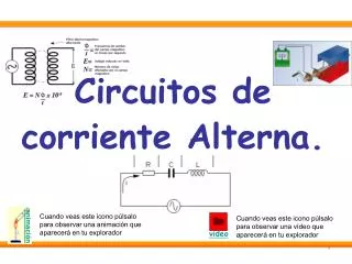
Corriente alterna
Corriente alterna. Generador de corriente alterna Valores eficaces Respuesta de los dipolos básicos Resistencia Autoinducción Condensador Circuito RLC serie Potencia de un dipolo RLC en serie Resistencia Autoinducción Condensador. Más. S. B. Generador de corriente alterna.

Corriente alterna
E N D
Presentation Transcript
Corriente alterna • Generador de corriente alterna • Valores eficaces • Respuesta de los dipolos básicos • Resistencia • Autoinducción • Condensador • Circuito RLC serie • Potencia de un dipolo RLC en serie • Resistencia • Autoinducción • Condensador Más
S B Generador de corriente alterna wt
Parámetros u(t) = Um cos(t + ) • Periodo T = 2/ • Frecuencia f = 1/T • Fase • Tensión máximaUm Um t T
Desfase entre intensidad y tensión i(t) = Im cost u(t) = Um cos(t + ) t
u2 t T Valores eficaces u Área media = 0 t T
Respuesta de los dipolos básicos Resistencia i(t) = Im cost u(t) = Um cost uR i R uR t i(t) uR = iR = ImRcost = 0
Autoinducción i(t) = Im cost u(t) = Um cos(t + p/2) uL i t L uL i(t) Um=LwIm XL = L Inductancia ()
Condensador i(t) = Im cost u(t) = Um cos(t - p/2) uC i t C uC i(t) XC = 1/C Capacitancia ()
Diagrama fasorial: resistencia i(t) = Im cos wt R uR(t) = R Im cos wt R Im Im
Diagrama fasorial: autoinducción i(t) = Im cos wt L XL Im XL = Lw Im p/2
Diagrama fasorial: condensador i(t) = Im cos wt C Xc = 1/Cw Im -p/2 XC Im
Ejemplo http://home.a-city.de/walter.fendt/physesp/physesp.htm
uR UL U UL - UC UR u uL UC uC Circuito RLC serie i = Imcost u = Umcos(t + ) R i(t) L I C Z: Impedancia
t = /4 t = t = 0 w w I1 I1 + I2 I2 I1 + I2 37º I1 37º I2 37º I1 + I2 I2 I1 w Fasores i1 = 4coswt i2 = 3cos(wt + 90º) i1 + i2 = 5cos(wt + 37º)
t Potencia de un dipolo RLC en serie i(t) = Imcost u(t) = Umcos(t + ) p(t) = i(t)u(t) = ImUmcostcos(t + ) p(t) = UeIe[cos (2t + ) + cos] * p u Pm =UeIecos i * 2cosAcosB = cos(A+B)+cos(A-B)
Potencia disipada en una resistencia UeR = IeR = 0 p(t) = Ie2R(1+cos2t) Pmedia = Ie2R pR t i uR
Potencia disipada en una autoinducción i UeL = IeL p(t)=LIe2cos(2t + /2) Pmedia = 0 t pL uL
Potencia disipada en un condensador UeC = Ie/C p(t)=CUe2cos(2t - /2) Pmedia = 0 uC pC i t
Potencia de un dipolo RLC en serie t i(t) = Im cost u(t) = Um cos(t + ) p(t) = ImUmcost cos(t + )
FORMA POLAR u U = 20 37º EXPRESIÓN INSTANTÁNEA Notación polar y binomial x = U cos y = U sen Um y x FORMA BINOMIAL u U = 20cos37º+20sen37ºj u U = 16 + 12j
u uu uuu U = Z I I = UY Ley de Ohm Ley de Ohm Z: Impedancia R: Resistencia X: Reactancia Y: Admitancia
UC = IXC –90º URL = I2XL 90º I1 I2 I2 URL UC I1 I XL I XC Diagramas fasoriales R ~
U1 0º IL1 IR I IR U2 I U2 = I XL2 90º IL1 –90º Diagramas fasoriales2 R L2 L1 U1 ~
18 A 45º Problema 15 VAB = 20IA - 6jIB IT= IA IB 10 2j A B 20 6j Tema siguiente